DDA3020 Machine Learning

Information Theory

Informaion

$I (x_{k}) = - lo g (p_{k})$

When $p_{k} = 1$ , $I (x_{k}) = 0$ , which means there is no uncertainty, then no information.

Entropy

Entropy is deﬁned as the expected value of information from a source.

$H_{p} (X) = E [I (x_{k})] = x_{k} \in X \sum p_{k} \cdot I (x_{k}) = - x_{k} \in X \sum p_{k} \cdot lo g (p_{k})$

Cross-entropy

Cross-entropy measures average bits needed to encode events from true distribution $P (X)$ using estimated distribution $Q (X)$ .

$H_{P, Q} (X) = E_{P} [I_{Q} (x)] = - x_{k} \in X \sum P (X = x_{k}) \cdot lo g (Q (X = x_{k}))$

Property 1 $H_{P, Q} (X) \geq 0$

Proof
$P (X = x_{k}) \in [0, 1], P (X = x_{k}) \in (0, 1] ⟹ H_{P, Q} \geq 0$ .

Property 2 $H_{P, Q} (X) \geq H_{P} (X)$

Proof

$H_{P, Q} (X) - H_{P} (X) = x_{k} \in X \sum P (x_{k}) lo g (\frac{P ( x _{k} )}{Q ( x _{k} )})$ By Jensen equality, for any convex function $f$ , $E [f (x)] \geq f (E [x])$ .
Since $lo g x$ is concave, we can implies $H_{P, Q} (X) - H_{P} (X) = - x_{k} \in X \sum P (x_{k}) lo g (\frac{Q ( x _{k} )}{P ( x _{k} )}) = E_{p} [- lo g (\frac{Q ( x _{k} )}{P ( x _{k} )})]$ Let $T = \frac{Q ( x )}{P ( x )}$ , then $E_{p} [- lo g T] \geq - lo g [E_{p} T] = - lo g [k \sum P (x_{k}) \frac{Q ( k )}{P ( x _{k} )}] = 0$ The equality holds only when $P = Q$ .

Kullback-Leibler divergence (KL-divergence)

The distance between two distributions.

$D_{K L} (P ∥ Q) = H_{P, Q} (X) - H_{P} (X) = \int_{x \in X} p_{X} (x) lo g (\frac{p _{X} ( x )}{q _{X} ( x )}) d x$

Property 1 $D_{K L} (P ∥ Q) \geq 0$

Proof $D_{K L} (P ∥ Q) = - \int_{x \in X} p_{X} (x) lo g (\frac{q _{X} ( x )}{p _{X} ( x )}) d x \geq - \int_{x \in X} p_{X} (x) (\frac{q _{X} ( x )}{p _{X} ( x )} - 1) d x = - \int_{x \in X} p_{X} (x) - q_{X} (x) d x = \int_{x \in X} q_{X} (x) d x - \int_{x \in X} p_{X} (x) d x = 0$

Property 2 $D_{K L} (P ∥ Q) \neq = D_{K L} (Q ∥ P)$

Linear Regression

Modeling of Linear Regression

Deterministic Perspective

Find $w$ which minimizes the following expression:

$\frac{1}{m} i = 1 \sum m (f_{w} (x_{i}) - y_{i})^{2}$

Probabilistic Perspective

$y = w^{⊤} x + e, where e \sim N (0, σ^{2})$

where $e$ is called obervation noise or residual error. The output $y$ can also be seen as a random variable, whose conditional probability is :

$p (y ∣ x, w) = N (w^{⊤} x, σ^{2})$

Given the training dataset $D = {(x_{i}, y_{i})}_{i = 1}^{m}$ , by maximum log-likehood estimaiton, we get

$lo g L (w; D) = lo g (i = 1 \prod m p (y_{i} ∣ x_{i}, w)) = i = 1 \sum m lo g N (w^{⊤} x, σ^{2}) = i = 1 \prod n lo g (\frac{1}{2 π σ ^{2}} exp (- \frac{( y _{i} - w ^{⊤} x _{i} ) ^{2}}{2 σ ^{2}})) = - m lo g (σ (2 π)^{\frac{1}{2}}) - \frac{1}{2 σ ^{2}} i = 1 \sum m (y_{i} - w^{⊤} x_{i})^{2}$

$w_{M L E} = arg max lo g L (w; D) = w arg min \frac{1}{2} i = 1 \sum m (y_{i} - w^{⊤} x_{i})^{2}$

Solutions of Linear Regression

Analytical solution

Let $e = Xw - y$ , then

$J (w) = i = 1 \sum m (f_{w} (x_{i}) - y_{i})^{2} = e^{⊤} e = w^{⊤} X^{⊤} Xw - 2 y^{⊤} Xw + y^{⊤} y$

Differentiating $J (w)$ with respect to $w$ and setting the result to $0$ :

$\frac{\partial}{\partial w} = 0 (X^{⊤} X is symmetric) ⟹ w^{⊤} X^{⊤} Xw = y^{⊤} Xw$

If $X^{⊤} X$ is invertible then $w = (X^{⊤} X)^{- 1} X^{⊤} y$

For linear regression with multiple outputs, $E = XW - Y$ , then

$J (W) = trace (E^{⊤} E)$

Gradient Descent

$J (w) = \frac{1}{2} i = 1 \sum m (y_{i} - w^{⊤} x_{i})^{2} = \frac{1}{2} ∥ Xw - y ∥^{2}$ , $w$ can be updated by gradient descent algorithm:

$w \leftarrow w - α \frac{\partial J ( w )}{\partial w} = w - α X^{⊤} (Xw - y)$

Classification

Binary Classification

If $X^{⊤} X$ is invertible then $w = (X^{⊤} X)^{- 1} X^{⊤} y$ , $f_{w} (x_{n e w}) = sgn (x_{n e w}^{⊤} w)$ .

Multi-Category Classification

Each ro in $Y$ has a one-hot assignment, then If $X^{⊤} X$ is invertible then $w = (X^{⊤} X)^{- 1} X^{⊤} Y$ , $f_{w} (x_{n e w}) = i = 1, \dots, C arg max (x_{n e w}^{⊤} W)$ .

Linear Regression Models

Ridge Regression

$J (w) = i = 1 \sum m (y_{i} - x_{i}^{⊤} w)^{2} + λ w^{⊤} w$

where $w = [0, w_{1}, w_{2}, \dots, w_{d}]^{⊤}$ (The bias $w_{0}$ should not be normalized).

To get $w min (Xw - y)^{⊤} (Xw - y) + λ w^{⊤} w$ ,

$\frac{\partial}{\partial w} (Xw - y)^{⊤} (Xw - y) + λ w^{⊤} w = 0 ⟹ w = (X^{⊤} X + λ \hat{I_{d}})^{- 1} X^{⊤} y (λ > 0)$ Where $\hat{I_{d}}$ is the identity matrix with the top-left element set to 0 to avoid penalizing the bias term $w_{0}$ .

We can assume that the parameter $w$ follow a zero-mean Gaussian prior $p (w) = N (w ∣ 0, τ^{2} I)$ (omit the bias $w_{0}$ ).

Utilizing this prior, we obtain the maximum a posteriori (MAP) estimation

$w_{M A P} z = p (w ∣ x, y) \propto p (y ∣ x, w) \cdot p (w) = w arg max [i = 1 \sum m lo g p (y_{i} ∣ x_{i}, w) + lo g p (w)] = w arg max [C - \frac{1}{2 σ ^{2}} i = 1 \sum m (y_{i} - x_{i}^{⊤} w)^{2} - \frac{1}{2 τ ^{2}} ∥ w ∥^{2}] \equiv w arg min [i = 1 \sum m (y_{i} - x_{i}^{⊤} w)^{2} + λ ∥ w ∥^{2}] (λ = \frac{σ ^{2}}{τ ^{2}})$

Polynomial Regression

$ϕ (x) = [1, x_{1}, \dots, x_{d}, \dots, x_{i} x_{j}, \dots, x_{i} x_{j} x_{k}, \dots]^{⊤} w = [w_{0}, w_{1}, \dots, w_{d}, \dots, w_{i, j}, \dots, w_{i, j, k}, \dots]^{⊤} f_{w} (x) = ϕ (x)^{⊤} w$

Note that $f_{w} (x)$ is still a linear function $w.r.t. w$ .

Lasso Regression

$p (w) = Lap (w ∣ 0, λ) = \frac{1}{2} exp (- \frac{∥ w ∥ _{1}}{λ})$ , then we have $w_{M A P} \equiv w arg min [i = 1 \sum m (y_{i} - x_{i}^{⊤} w)^{2} - α ∥ w ∥_{1}]$ .

Ridge uses L2 penalty, shrinking weights towards zero without feature selection. In contrast, Lasso uses L1 penalty, forcing some weights to exactly zero, achieving model sparsity and automatic feature selection.

Robust Linear Regression

Adpot the $l_{1}$ loss as follows $J (w) = i = 1 \sum m ∣ x_{i}^{⊤} w - y_{i} ∣$ .

Assuming that $p (y ∣ x, w, b) = (y ∣ w^{⊤} x, b) \propto exp (- \frac{1}{b} ∣ y - w^{⊤} x ∣)$ , $w_{M L E} \equiv w arg min \frac{1}{b} i = 1 \sum m ∣ x_{i}^{⊤} w - y_{i} ∣$ .

Two ways to make it differentiable:

$w, t min i \sum m t_{i} s.t. - t_{i} \leq x_{i}^{⊤} w - y_{i} \leq t_{i}, 1 \leq i \leq m$ .
By using the following equation $∣ a ∣ = μ > 0 min \frac{1}{2} (\frac{a ^{2}}{μ} + μ)$ .

Then it can be reformulated as follows:

$w min μ_{1}, \dots, μ_{m} > 0 min \frac{1}{2} i = 1 \sum m (\frac{( x _{i}^{⊤} w - y _{i} ) ^{2}}{μ _{i}} + μ_{i})$

Given $w$ , $μ_{i} = ∣ x_{i}^{⊤} w - y_{i} ∣$ ; Given $μ$ , $w = w arg min i = 1 \sum m \frac{1}{2} \frac{( x _{i}^{⊤} w - y _{i} ) ^{2}}{μ _{i}}$ .

Comparison

$p (y ∣ x, w)$	$p (w)$	Regression Method
Gaussian	Uniform	Least squares
Gaussian	Gaussian	Ridge regression
Gaussian	Laplace	Lasso regression
Laplace	Uniform	Robust regression
Student	Uniform	Robust regression

Logistic Regression

Hypothesis Function

$f_{w} (x) = P (y = 1 ∣ x; w) = g (w^{⊤} x) \in [0, 1] g (z) = \frac{1}{1 + exp ( - z )} g^{'} (z) = g (z) (1 - g (z))$

The decision boundary satisfies $g (z) \geq 0.5$ when $z \geq 0$ , and $g (z) < 0.5$ when $z < 0$ , $i.e.$ , it is determined by $w^{⊤} x + b = 0$ .

Cost Function

$ℓ_{2}$ Loss
- Linear Regression
  
  $J (w) = \frac{1}{2 m} i = 1 \sum m (f_{w} (x_{i}) - y_{i})^{2} = \frac{1}{2 m} ∥ Xw - y ∥^{2}$ , $H = \nabla_{w}^{2} J (w) = \frac{1}{m} X^{⊤} X ⪰ 0 ⟹ convex$
- Logistic Regression
  
  $J (w) = \frac{1}{2 m} i = 1 \sum m (g (w^{⊤} x_{i}) - y_{i})^{2} ⟹ non-convex$
Cross-entropy Loss

$cost (y (x), f_{w} (x)) = - P (y = 1 ∣ x) \cdot lo g P (y = 1 ∣ x; w) - P (y = 0 ∣ x) \cdot P (y = 0 ∣ x; w) = {- lo g (f_{w} (x)) y (x) = 1 - lo g (1 - f_{w} (x)) y (x) = 0$

$J (w) = \frac{1}{m} i = 1 \sum m cost (y_{i}, f_{w} (x_{i}))$

For $y_{i} = 1, J_{i} (w) = - lo g (σ_{i})$ , $\nabla_{w} J_{i} = - (1 - σ_{i}) x_{i}$ , $\nabla_{w}^{2} J_{i} = σ_{i} (1 - σ_{i}) x_{i} x_{i}^{⊤}$ .

For $y_{i} = 0, J_{i} (w) = - lo g (1 - σ_{i})$ , $\nabla_{w} J_{i} = σ_{i} \cdot x_{i}$ , $\nabla_{w}^{2} J_{i} = σ_{i} (1 - σ_{i}) x_{i} x_{i}^{⊤}$ .

$⟹ J (w) convex$

Gradient Descent

Assume $m$ samples in total. Learning $w$ by minimizing $J (w)$

$w^{*} = w arg min J (w) = - \frac{1}{m} i = 1 \sum m [y_{i} lo g (f_{w} (x_{i})) + (1 - y_{i}) lo g (1 - f_{w} (x_{i}))]$

By gradient descent

$w \leftarrow w - α \nabla J (w) = w - \frac{α}{m} i = 1 \sum m [\frac{y _{i}}{f _{w} ( x _{i} )} \cdot \nabla f_{w} (x_{i}) + \frac{1 - y _{i}}{1 - f _{w} ( x _{i} )} \cdot \nabla f_{w} (x_{i})] = w - \frac{α}{m} i = 1 \sum m [\frac{y _{i}}{f _{w} ( x _{i} )} - \frac{1 - y _{i}}{1 - f _{w} ( x _{i} )}] \cdot [f_{w} (x_{i}) (1 - f_{w} (x_{i}))] \cdot x_{i} = w - \frac{α}{m} i = 1 \sum m [f_{w} (x_{i}) - y_{i}] \cdot x_{i}$

Multi-class Classification

Softmax

$f_{W}^{(j)} (x) = \frac{exp w _{j}^{⊤} x}{c = 1 \sum C exp ( w _{c}^{⊤} x )} = P (y = j ∣ x, W)$

$\frac{\partial f _{w_{c}}}{\partial w _{j}} = {f_{w_{j}} (1 - f_{w_{j}}) x_{i} c = j - f_{w_{j}} f_{w_{c}} x_{i} c \neq = j$

Cost Function

$J (W) = - \frac{1}{m} i \sum m j \sum C [I (y_{i} = j) lo g (f_{w_{j}} (x_{i}))]$

$\frac{\partial J ( W )}{\partial w _{j}} = - \frac{1}{m} i \sum m \frac{I ( y _{i} = j )}{f _{w_{j}} ( x _{i} )} \cdot \frac{\nabla f _{w_{j}} ( x _{i} )}{\nabla w _{j}} + c \neq = j \sum C \frac{I ( y _{i} = c )}{f _{w_{c}} ( x _{i} )} \cdot \frac{\nabla f _{w_{c}} ( x _{i} )}{\nabla w _{j}} ⟹ \frac{1}{m} i \sum m (f_{w_{j}} (x_{i}) - I (y_{i} = j)) x_{i}$

Regularized Logistic Regression

$\overline{J} (w) = J (w) + \frac{λ}{2 m} j = 1 \sum d w_{j}^{2} = - \frac{1}{m} i \sum m [y_{i} lo g f_{w} (x_{i}) + (1 - y_{i}) lo g (1 - f_{w} x_{i})] + \frac{λ}{2 m} i = 1 \sum d w_{j}^{2}$

$w_{0} \leftarrow w_{0} - α \frac{\partial J ( w )}{\partial w _{j}} = w_{j} - \frac{α}{m} i = 1 \sum m (f_{w} (x_{i}) - y_{i}) x_{i} (0) where x_{i} (0) = 1$

Linear Regression vs Logistic Regression

Dimension	Linear Regression	Logistic Regression
Task Type	Regression task predicting continuous real values	Classification task predicting discrete class labels
Model Hypothesis	Linear function $f_{w} (x) = w^{⊤} x$ Output range $(- \infty, + \infty)$	Sigmoid-mapped linear function $f_{w} (x) = g (w^{⊤} x)$ Output range $[0, 1]$ (posterior probability of positive class)
Loss Function	Residual sum of squares (MSE) $\frac{1}{2 m} i = 1 \sum m (y_{i} - w^{⊤} x_{i})^{2}$	Cross-entropy loss $- \frac{1}{m} i = 1 \sum m [y_{i} lo g f_{w} (x_{i}) + (1 - y_{i}) lo g (1 - f_{w} (x_{i}))]$
Solution Method	Closed-form solution $w^{*} = (X^{⊤} X)^{- 1} X^{⊤} y$ or gradient descent	No closed-form solution, optimized via gradient descent

Supoort Vector Machine

Larger Marigin

Denote $f_{w, b} (x) = w^{⊤} x + b = 0$ is a hyperplane, then $w$ is orthogonal to the hyperplane, and $x$ has the distance $\frac{∣ f _{w, b} ( x ) ∣}{∥ w ∥}$ to the hyperplane.

Margin is defined as the distance between the hyperplane and the closest data point, which can be formulated as $γ = i min \frac{y _{i} f _{w, b} ( x )}{∥ w ∥}$ with $y_{i} \in {- 1, 1}$ .

Since $w, b max γ = w, b max i min \frac{y _{i} f _{w, b} ( x )}{∥ w ∥}$ . Set $y_{i} f_{w, b} (x) = 1$ , then $γ = \frac{1}{∥ w ∥}$ ,

Then the optimization problem can be formulated as follows:

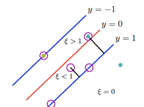
$w, b min \frac{1}{2} ∥ w ∥^{2} s.t. y_{i} (w^{⊤} x_{i} + b) \geq 1, i = 1, 2, \dots, m$

Hinge Loss

Let $f_{w, b} (x) = \frac{1}{1 + exp - ( w ^{⊤} x + b )} = g (z)$ where $z = w^{⊤} x + b$ be the hypothesis function, then the cost function can be defined as follows:

$J (w) = \frac{1}{m} i \sum m [- δ_{y = 1} lo g (f_{w, b} (x)) - δ_{y = - 1} lo g (1 - f_{w, b} (x))] + \frac{λ}{2 m} j = 1 \sum n w_{j}^{2} \equiv C \cdot \frac{1}{m} i \sum m [- δ_{y = 1} lo g (f_{w, b} (x)) - δ_{y = - 1} lo g (1 - f_{w, b} (x))] + \frac{1}{2} j = 1 \sum n w_{j}^{2} (C = \frac{1}{λ})$

The hinge loss is defined as follows

$max (0, 1 - y_{i} (w^{⊤} x_{i} + b))$

Then the optimization problem can be reformulated as follows

$w, b min C \cdot i \sum m max (0, 1 - y_{i} (w^{⊤} x_{i} + b)) + \frac{1}{2} j = 1 \sum n w_{j}^{2}$

Largrange Duality

The objective function of SVM is

$w, b min \frac{1}{2} ∥ w ∥^{2} s.t. y_{i} (w^{⊤} x_{i} + b) \geq 1, i = 1, 2, \dots, m$

Its Lagrangian function is defined as follows

$L (w, b, α) = \frac{1}{2} ∥ w ∥^{2} - i = 1 \sum m α_{i} [1 - y_{i} (w^{⊤} x_{i} + b)]$

The KKT conditions are as follows

$⎩ ⎨ ⎧ Stationarity ⎩ ⎨ ⎧ \frac{\partial L ( w , b , α )}{\partial w} = 0 ⟹ w = i = 1 \sum m α_{i} y_{i} x_{i} \frac{\partial L ( w , b , α )}{\partial b} = 0 ⟹ i = 1 \sum m α_{i} y_{i} = 0 Feasibility α_{i} \geq 0, 1 - y_{i} (w^{⊤} x_{i} + b) \leq 0, \forall i Complementary Slackness α_{i} \cdot (1 - y_{i} (w^{⊤} x_{i} + b)) = 0, \forall i$

Then the Largangian function can be reformulated as follows

$L (w, b, α) = \frac{1}{2} ∥ w ∥^{2} + i = 1 \sum m α_{i} - i = 1 \sum, α_{i} y_{i} (j = 1 \sum m α_{j} y_{j} x_{j})^{⊤} x_{i} - i = 1 \sum m α_{i} y_{i} b = i = 1 \sum m α_{i} - \frac{1}{2} i = 1 \sum m j = 1 \sum m α_{i} α_{j} y_{i} y_{j} x_{i}^{⊤} x_{j}$

Then the dual problem is obtained as follows

$α max i = 1 \sum m α_{i} - \frac{1}{2} i = 1 \sum m j = 1 \sum m α_{i} α_{j} y_{i} y_{j} x_{i}^{⊤} x_{j} s.t. α_{i} \geq 0, i = 1 \sum m α_{i} y_{i} = 0, \forall i$

The data points with $α_{i} > 0$ are called support vectors, which locate on the margin and determine the decision boundary. Let $S = {i ∣ α_{i} > 0}$ be the set of support vectors, then the decision boundary can be determined by any support vector as follows:

$y_{i} (w^{⊤} x_{i} + b) = 1 ⟹ b = \frac{1}{∣ S ∣} i \in S \sum (y_{i} - w^{⊤} x_{i}) = \frac{1}{∣ S ∣} i \in S \sum (y_{i} - j = 1 \sum m α_{j} y_{j} x_{i}^{⊤} x_{j})$

SVM with Slack Variables

In this case, the optimization problem can be formulated as follows

$w, b, ξ min \frac{1}{2} ∥ w ∥^{2} + C i = 1 \sum m ξ_{i} s.t. 1 - ξ_{i} - y_{i} (w^{⊤} x_{i} + b) \leq 0, - ξ_{i} \leq 0, \forall i$

Its Lagrangian function is defined as follows

$L (w, b, ξ, α, β) = \frac{1}{2} ∥ w ∥^{2} + C i = 1 \sum m ξ_{i} - i = 1 \sum m α_{i} (1 - ξ_{i} - y_{i} (w^{⊤} x_{i} + b)) - i = 1 \sum m β_{i} (- ξ_{i})$

The KKT conditions are as follows

$⎩ ⎨ ⎧ Stationarity ⎩ ⎨ ⎧ \frac{\partial L ( w , b , ξ , α , β )}{\partial w} = 0 ⟹ w = i = 1 \sum m α_{i} y_{i} x_{i} \frac{\partial L ( w , b , ξ , α , β )}{\partial b} = 0 ⟹ i = 1 \sum m α_{i} y_{i} = 0 \frac{\partial L ( w , b , ξ , α , β )}{\partial ξ _{i}} = 0 ⟹ α_{i} + β_{i} = C, \forall i Feasibility α_{i} \geq 0, β_{i} \geq 0, 1 - ξ_{i} - y_{i} (w^{⊤} x_{i} + b) \leq 0, - ξ_{i} \leq 0, \forall i Complementary Slackness α_{i} \cdot (1 - ξ_{i} - y_{i} (w^{⊤} x_{i} + b)) = 0, β_{i} \cdot (- ξ_{i}) = 0, \forall i$

The the Lagrange function can be reformulated as follows

$L (α, β) = i = 1 \sum m α_{i} - \frac{1}{2} i = 1 \sum m j = 1 \sum m α_{i} α_{j} y_{i} y_{j} x_{i}^{⊤} x_{j}$

The dual problem can be reformulated as follows

$α max i = 1 \sum m α_{i} - \frac{1}{2} i = 1 \sum m j = 1 \sum m α_{i} α_{j} y_{i} y_{j} x_{i}^{⊤} x_{j} s.t. 0 \leq α_{i} \leq C, i = 1 \sum m α_{i} y_{i} = 0, \forall i$

Let $M = {i ∣ 0 < α_{i} < C}$ . The bias parameter $b$ can be determined by any support vector with $0 < α_{i} < C$ as follows

$i = 1 \sum m α_{i} y_{i} x_{i}^{⊤} x_{j} + b = y_{j}, where j \in M ⟹ b = \frac{1}{∣ M ∣} j \in M \sum (y_{j} - i = 1 \sum m α_{i} y_{i} x_{i}^{⊤} x_{j})$

Condition on $α_{i}$	Slack $ξ_{i}$	Contributes to classifier?	Correctly classified?	Location relative to margin / decision boundary
$α_{i} = 0$	$0$	No	Yes	Outside the margin
$0 < α_{i} < C$	$0$	Yes	Yes	On the margin
$α_{i} = C$	$0 \leq ξ_{i} \leq 1$	Yes	Yes	Inside the margin, not crossing decision boundary
$α_{i} = C$	$ξ_{i} > 1$	Yes	No	Crossing decision boundary

SVM with Kernels

Define the kernel function $k (x_{i}, x_{j}) = ϕ (x_{i})^{⊤} ϕ (x_{j})$ , then the dual problem can be reformulated as follows

$α max i = 1 \sum m α_{i} - \frac{1}{2} i = 1 \sum m j = 1 \sum m α_{i} α_{j} y_{i} y_{j} k (x_{i}, x_{j}) s.t. α_{i} \geq 0 i = 1 \sum m α_{i} y_{i} = 0, \forall i$

The solution $b$ becomes

$b = \frac{1}{∣ S ∣} j \in S \sum (y_{j} - i = 1 \sum m α_{i} y_{i} k (x_{i}, x_{j}))$

The prediction of new data $x$ becomes

$w^{⊤} ϕ (x) + b = i = 1 \sum m α_{i} y_{i} k (x_{i}, x) + b$

Some kernel functions

$⎩ ⎨ ⎧ Polynomial kernel k (x_{i}, x_{j}) = (1 + \frac{x _{i}^{⊤} x _{j}}{σ ^{2}})^{p}, p > 0 Gaussian RBF kernel k (x_{i}, x_{j}) = exp (- \frac{∥ x _{i} - x _{j} ∥ ^{2}}{2 σ ^{2}}) Sigmoid kernel k (x_{i}, x_{j}) = \frac{1}{1 + exp ( - γ x _{i}^{⊤} x _{j} + c )}$

Multi-class SVM

Predict the label of $x$ as $k \in {1, 2, \dots, K} arg max (w^{(k)})^{⊤} x + b^{(k)}$ , $i.e.$ , use one-vs-rest strategy to train $K$ binary SVM classifiers.

Tree-based Methods

Decsion Tree

A decision tree (non-parametric model) is a hierarchical model for supervised learning whereby the local region is identified in a sequence of recursive splits.

Classification Tree

Impurity Measure (Choose the attribute that maximizes the reduction in impurity.)

Let $S_{i}$ be the seef of instances of $S$ belonging to class $C_{i}$ ( $i = 1, 2, \dots, K$ ), then $\hat{P} (C_{i} ∣ x, S) \equiv p_{i} = \frac{∣ S _{i} ∣}{∣ S ∣}$ is the proportion of class $C_{i}$ in $S$ .

Entropy is the measurement of impurity, which is defined as follows

$Info (S) = - i = 1 \sum K p_{i} lo g p_{i}$

And the entropy of $S$ given the condition of attribute $A$ is defined as follows (Suppose attribute $A \in {a_{1}, a_{2}, \dots, a_{V}}$ to split $S$ into $V$ subsets $D_{1}, D_{2}, \dots, D_{V}$ )

$Info (S ∣ A) = v = 1 \sum V \frac{∣ S _{v} ∣}{∣ S ∣} Info (D_{v})$

Information gained by branching on atribute $A$ is defined as follows

$Gain (A) = Info (S) - Info (S ∣ A)$
Gini Index

Gini index is another measurement of impurity, which is defined as follows

$Gini (S) = 1 - i = 1 \sum K p_{i}^{2}$

It means the probability of different class labels for two randomly selected instances from $S$ .

And the Gini index of $S$ given the condition of attribute $A$ is defined as follows (Suppose attribute $A \in {a_{1}, a_{2}, \dots, a_{V}}$ to split $S$ into $V$ subsets $D_{1}, D_{2}, \dots, D_{V}$ )

$Gini (S ∣ A) = v = 1 \sum V \frac{∣ S _{v} ∣}{∣ S ∣} Gini (D_{v})$

Gini gain by branching on atribute $A$ is defined as follows

$Δ Gini (A) = Gini (S) - Gini (S ∣ A)$

Regression Tree

The regression tree grows by recursively selecting the binary split on any variable that most reduces the sum of squared errors.

$\overline{y}_{c} = \frac{i \in c \sum y _{i}}{N _{c}}$ is the prediction for leaf $c$ , where $N_{c}$ is the number of instances in leaf $c$ .

Mean Squared Error (MSE)

$MSE (c) = \frac{1}{N _{c}} i \in c \sum (y_{i} - \overline{y}_{c})^{2}$

The total MSE is $S = c \in leaves \sum MSE (c)$ .
Sum of squared Errors (SSE)

The total SSE is $S = c \in leaves \sum i \in c \sum (y_{i} - \overline{y}_{c})^{2}$ .

Overfitting and Pruning

Pruning of the decision tree is one by replacing a subtree with a leaf node. The subtree is replaced if the error of the subtree on the validation set is larger than the error of the leaf node on the validation set.

Ensemble Models

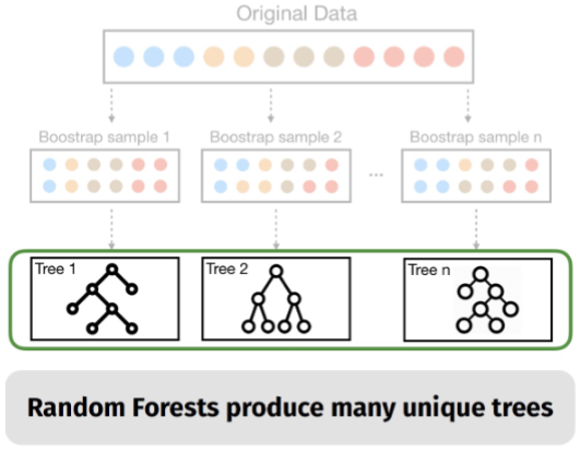
Bagging

Sample records with replacement from the training set to create multiple bootstrap samples, and train a base model on each bootstrap sample. The final prediction is obtained by averaging the predictions of all base models.

It aggreates the predictions of all single trees and produces many correlated trees, which the diversity of the trees is not high.

Random Forest

It chooses a random subset of features to split each node, which increases the diversity of the trees and reduces the correlation between trees.

Neural Networks

Activation Function

Perceptron Model

$y = f (w^{⊤} x + b) = Sign (w^{⊤} x + b)$ , the objective function is $J (w) = \frac{1}{2} (y - t)^{2}$ , and the update rule is $w \leftarrow w - η (y - t) x$ .

For a new data point $x$ , the prediction is $y = Sign (w^{⊤} x + b)$ , which is a linear classifier.

Multi-layer Feedforward Neural Networks

To solve XOR, a one‑hidden‑layer network learns non‑linear input features. Each layer re‑expresses the previous layer’s output, progressively extracting more abstract and discriminative features.

$y = f^{(L)} \circ f^{(L - 1)} \circ \dots \circ f^{(1)} (x)$ , where $f^{(l)} (z) = g (W^{(l)} z + b^{(l)})$ is the transformation of layer $l$ .

Backpropagation (using computational graph (CG))

Forward Pass

For each $i = 1, \dots, N$ , compute $v_{i}$ as a function of its parents.

Backward Pass

$\overline{v}_{N} = 1$ , then for $i = N - 1, \dots, 1$ , $\overline{v}_{i} = j \in children (i) \sum \overline{v}_{j} \cdot \frac{\partial v _{j}}{\partial v _{i}}$ . Also update parameters $w, b$ by

$w \leftarrow w - η \cdot \frac{\partial C _{i}^{(n + 1)}}{\partial w _{i}^{(n)}} b \leftarrow b - η \cdot \frac{\partial C _{i}^{(n + 1)}}{\partial b _{i}^{(n)}}$

where $C_{i}^{(n + 1)}$ is the cost function of layer $n + 1$ .

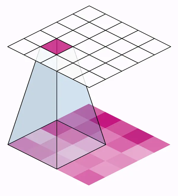
Convolutional Neural Networks

Convolutional Layer

$f \circ g (x) = \int f (t) g (x - t) d t$

Input volume is $W_{1} \times H_{1} \times C$ .

A convolutional layer has four hyperparameters: number of filters $K$ , filter size $F$ , stride $S$ , and zero padding $P$ (per side).

Output spatial size is $W_{2} = ⌊ \frac{W _{1} - F + 2 P}{S} ⌋ + 1$ and $H_{2} = ⌊ \frac{H _{1} - F + 2 P}{S} ⌋ + 1$ .

Output volume is $W_{2} \times H_{2} \times K$ .

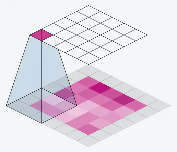
Number of parameters is $F^{2} C K$ weights plus $K$ biases. parameters is $F^{2} C K$ weights plus $K$ biases.

Pooling Layer

Pooling layer has no learnable parameters. Hyperparameters are filter size $F$ and stride $S$ .

Output spatial size is $W_{2} = ⌊ \frac{W _{1} - F}{S} ⌋ + 1$ and $H_{2} = ⌊ \frac{H _{1} - F}{S} ⌋ + 1$ .

Pooling operates on each channel independently, so output volume is $W_{2} \times H_{2} \times C$ .

Common pooling functions are $Max$ and $Average$ .

Fully Connected Layer

A fully connected layer computes the class scores, resulting in an output volume of $1 \times 1 \times N_{c}$ , where $N_{c}$ is the number of classes, which contains neurons that connect to the entire input volume.

Recurrent Neural Networks and Transformer

RNN

Basic

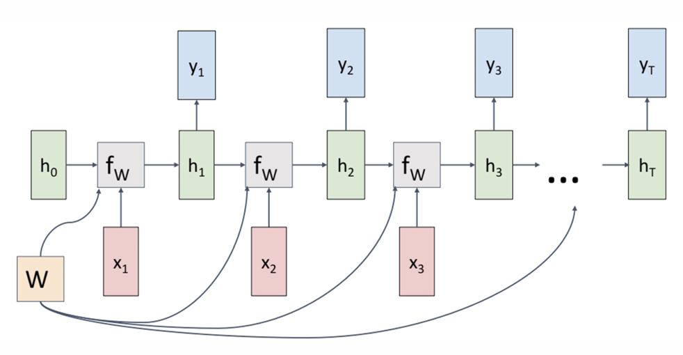
$h_{t} = f_{W} (h_{t - 1}, x_{t})$ , $\overset{y}{^}_{t} = g_{W^{'}} (h_{t})$ , where $f_{W}$ is the transition function and $g_{W^{'}}$ is the output function. The cost/error function is $E (θ) = \frac{1}{T} t = 1 \sum T L (\overset{y}{^}_{t}, y_{t})$ , where $θ = {W, W^{'}}$ .

However, the basic RNN suffers from vanishing/exploding gradient problem, which makes it difficult to learn long-term dependencies.

Long Short-Term Memory (LSTM)

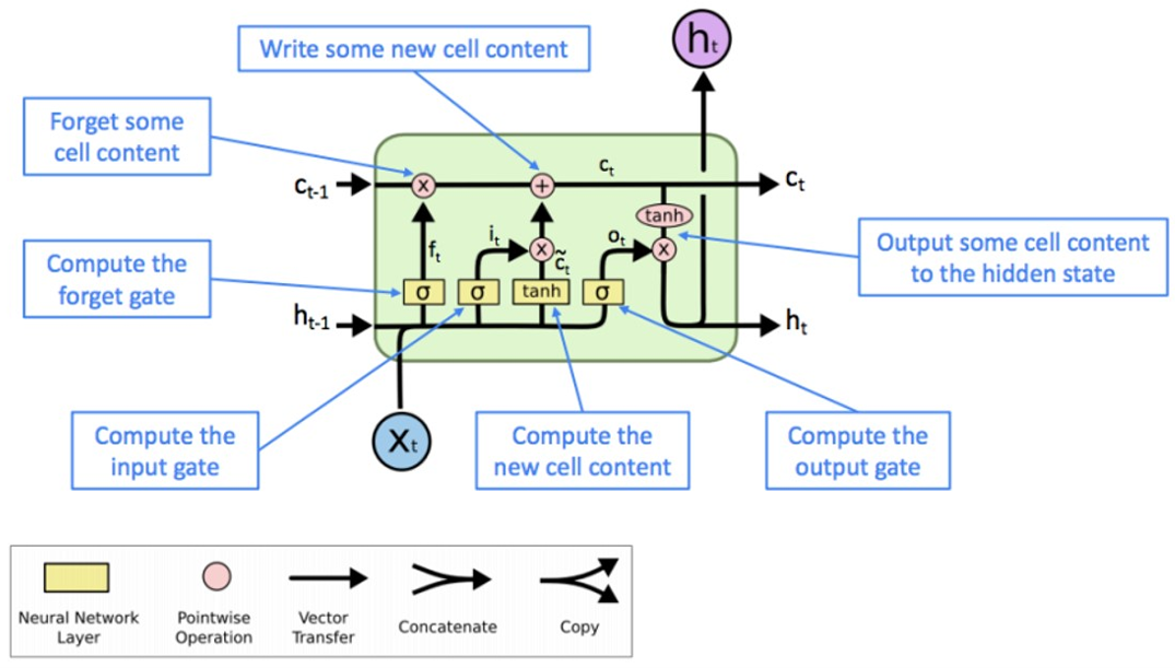
Limitations

Difficulty with Long-Term Dependencies
Limited Parallelization

Transformer

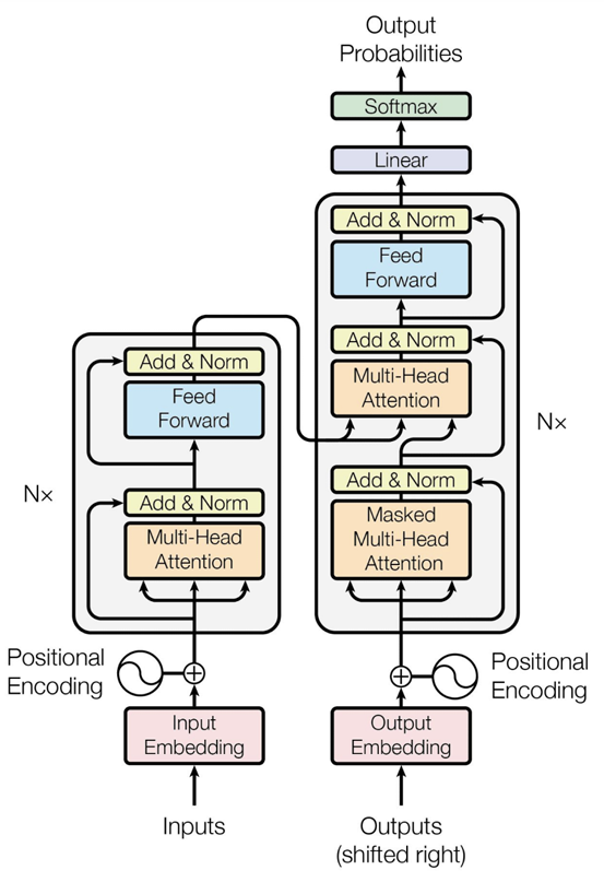
Attention Mechanism

Let $Q = X W_{Q}, K = X W_{K}, V = X W_{V}$ be the query, key, and value matrices, where $W_{Q}, W_{K}, W_{V} \in R^{d \times d^{'}}$ and $X \in R^{n \times d}$ is the input sequence. Then the attention output is defined as follows

$Z = attention(Q, K, V) = softmax (\frac{Q K ^{⊤}}{d ^{'}}) V$

Multi-head Attention

Multi-head attention allows the model to jointly attend to information from different representation subspaces at different positions, capturing diverse types of relationships in parallel.

Bias-variance Tradeoff

Let $D$ be training dataset drawn $i.i.d.$ from $P^{n}$ , $h_{D} = A (D)$ be the model trained by algorithm $A$ on $D$ .

$\overset{ˉ}{h} = E_{D \sim P^{n}} [h_{D}] = \int_{D} h_{D} p (D) d D$

expected test error for a fixed model $h_{D}$ $E_{(x, y) \sim P} [(h_{D} (x) - y)^{2}] = \int_{x} \int_{y} (h_{D} (x) - y)^{2} p (x, y) d x d y$ .
expected test error for the algorithm $A$ $E_{(x) \sim P, D \sim P^{n}} [(h_{D} (x) - y)^{2}] = \int_{D} \int_{x} \int_{y} (h_{D} (x) - y)^{2} p (x, y) p (D) d x d y d D$ .
the expected test error $E_{(x, y), D} [(h_{D} (x) - y)^{2}]$ . (mean squared error (MSE))

$E_{(x, y), D} [(h_{D} - \overset{ˉ}{h}) (\overset{ˉ}{h} - y)] = E_{(x, y)} [E_{D} [h_{D} - \overset{ˉ}{h}] \cdot (\overset{ˉ}{h} - y)] = E_{(x, y)} [(E_{D} [h_{D}] - \overset{ˉ}{h}) \cdot (\overset{ˉ}{h} - y)] = E_{(x, y)} [(\overset{ˉ}{h} - \overset{ˉ}{h}) \cdot (\overset{ˉ}{h} - y)] = 0$

$E_{(x, y), D} [(h_{D} (x) - y)^{2}] = E [(h_{D} - \overset{ˉ}{h})^{2}] + 2 E [(h_{D} - \overset{ˉ}{h}) (\overset{ˉ}{h} - y)] + E [(\overset{ˉ}{h} - y)^{2}] = E_{(x, y), D} [(h_{D} - \overset{ˉ}{h})^{2}] + E_{(x, y), D} [(\overset{ˉ}{h} - y)^{2}]$

Now decompose the second term $E [(\overset{ˉ}{h} - y)^{2}]$ , $y = t (x) + ϵ, ϵ \sim N (0, σ^{2})$ .

$E_{(x, y)} [(\overset{ˉ}{h} - t (x)) (t (x) - y)] = E_{x} [E_{y ∣ x} [(\overset{ˉ}{h} (x) - t (x)) (t (x) - y)]] = E_{x} [(\overset{ˉ}{h} (x) - t (x)) \cdot E_{y ∣ x} [t (x) - y]] = E_{x} [(\overset{ˉ}{h} (x) - t (x)) \cdot (t (x) - E [y ∣ x])] = E_{x} [(\overset{ˉ}{h} (x) - t (x)) \cdot (t (x) - t (x))] = 0$

$E [(\overset{ˉ}{h} - y)^{2}] = E [(\overset{ˉ}{h} - t (x))^{2}] + 2 E [(\overset{ˉ}{h} - t (x)) (t (x) - y)] + E [(t (x) - y)^{2}]$

$⟹ E_{(x, y), D} [(h_{D} (x) - y)^{2}] = Variance E_{(x, y), D} [(h_{D} (x) - \overset{ˉ}{h} (x))^{2}] + Bias^{2} E_{(x, y)} [(\overset{ˉ}{h} (x) - t (x))^{2}] + Noise E_{(x, y)} [(t (x) - y)^{2}]$

Comparsion

Term	Description
Variance	Measures how much the predictions of a model vary when trained on different training sets. (model's sensitivity to the specific training data)
Bias²	Measures how far the average prediction of a model is from the true value. (model's systematic error)
Noise	Measures how much the observed values vary around the true target function due to randomness in the data. (data's inherent unpredictability)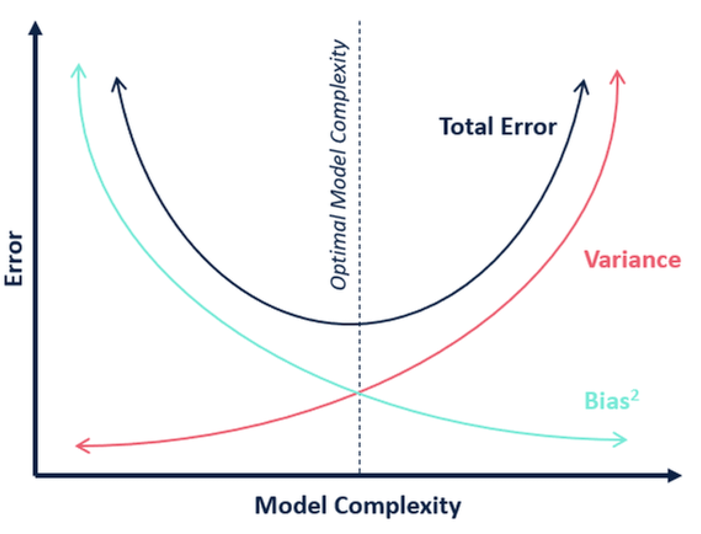

Performance Evaluation

Hyper-parameter Tuning

Determined typically outside the learning algorithms rather than earned by a learning algorithm based on the trainingset.

Cross-validation

Cross-validation is a statistical method of evaluating generalization performance that is more stable and thorough than using a split into a training and a test set.

K-fold cross validation

Split the train data into $K$ folds, try each fold as validation, while other folds as train. Note that $K$ is a hyper-parameter.

Evaluation Metrics

Regression

Mean Square Error $\frac{i = 1 \sum n ( y _{i} - y _{i} ) ^{2}}{n}$
Mean Absolute Error $\frac{i = 1 \sum n ∣ y _{i} - y _{i} ∣}{n}$

Classification

Confusion Matrix

Actual \ Predicted $P$ (Predicted) $N$ (Predicted)

$P$ (Actual) $TP$ $FN$

$N$ (Actual) $FP$ $TN$
- Accuracy The total number of correctly classiﬁed samples over all samples under evaluation.
  
  $\frac{TP + TN}{TP + TN + FP + FN}$
- Precision The proportion of correctly predicted positive samples among all samples predicted as positive.
  
  $\frac{TP}{TP + FP}$
- Recall The proportion of correctly predicted positive samples among all actual positive samples.
  
  $\frac{TP}{TP + FN}$
- Cost-sensitive Accuracy (different classes may have different importance)
  
  $Cost-Sensitive Accuracy = \frac{C _{p, p} \cdot TP + C _{n, n} \cdot TN}{C _{p, p} \cdot TP + C _{n, n} \cdot TN + C _{p, n} \cdot FN + C _{n, p} \cdot FP}$
- Binary Classification
  
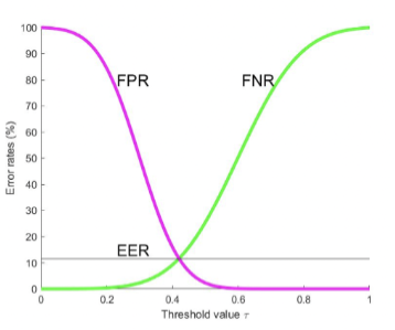
  Metric Formula
  
  $TPR$ (True Positive Rate) $\frac{TP}{TP + FN}$
  
  $FNR$ (False Negative Rate) $\frac{FN}{TP + FN}$
  
  $TNR$ (True Negative Rate) $\frac{TN}{FP + TN}$
  
  $FPR$ (False Positive Rate) $\frac{FP}{FP + TN}$
  
  If positive and negative classes are balanced, then $Accuracy = \frac{TPR + TNR}{2} = 1 - \frac{FPR + FNR}{2}$ .
  
  As the decision threshold varies from $0$ to $1$ , FPR decreases while FNR increases, and their intersection point where $FPR$ equals $FNR$ is called the Equal Error Rate ( $EER$ ). The lower the $EER$ , the better the classifier.
Receiver Operating Characteristic Curve (ROC) The relationship between FNR and FPR.
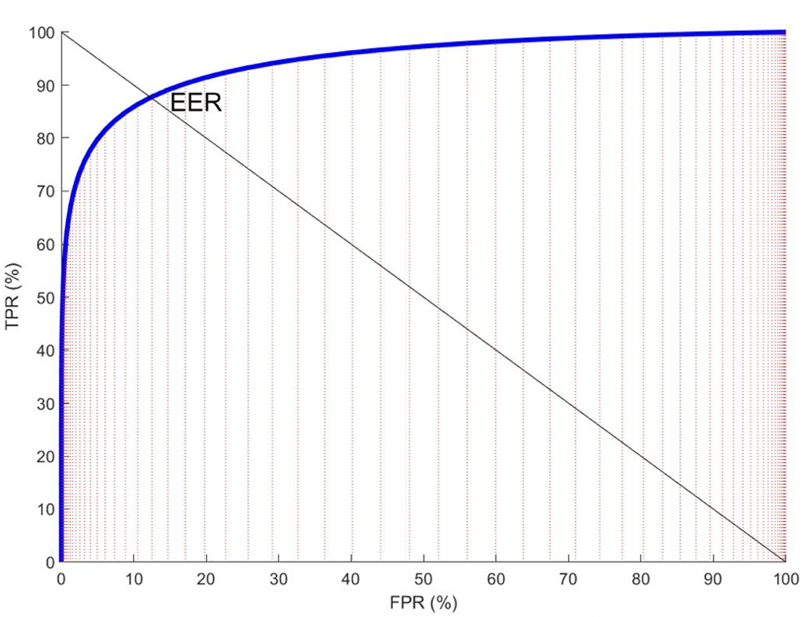
Area Under the ROC (AUC) The probability that a randomly chosen positive example is ranked higher than a randomly chosen negative example. (It means the perfect prediction if it equals to $1$ .)

Consider a set of binary samples indexed by $i = 1, \dots, m^{+}$ for positive class, $j = 1, \dots, m^{-}$ and for negative class. Let $g (x)$ be a predictor and $e_{ij} = g (x_{i}^{+}) - g (x_{j}^{-})$ .

Consider also a Heaviside step function given by

$u (e) = ⎩ ⎨ ⎧ 0, 0.5, 1, x < 0 x = 0 x > 0$

Then AUC can be expressed by $AUC = \frac{1}{m ^{+} m ^{-}} i = 1 \sum m^{+} j = 1 \sum m^{-} u (e_{ij})$ .

Actual \ Predicted	$P$ (Predicted)	$N$ (Predicted)
$P$ (Actual)	$TP$	$FN$
$N$ (Actual)	$FP$	$TN$

Metric	Formula
$TPR$ (True Positive Rate)	$\frac{TP}{TP + FN}$
$FNR$ (False Negative Rate)	$\frac{FN}{TP + FN}$
$TNR$ (True Negative Rate)	$\frac{TN}{FP + TN}$
$FPR$ (False Positive Rate)	$\frac{FP}{FP + TN}$

Unsupervised Learning

Clustering

Clustering is a problem of learning to assign labels to examples by leveraging an unlabeled dataset.

Dimensionality Reduction

Principal componentanalysis (PCA) is a technique that converts a set of observations of possibly correlated variables into a set of values of linearly uncorrelated variables, called principal components.

Density Estimation

Estimate the distribution based on some observed data.

Kernel Density Estimation (KDE)

$\hat{f}_{b} (x) = \frac{1}{N b} i = 1 \sum N k (\frac{x - x _{i}}{b}) k (z) = \frac{1}{2 π} exp (- \frac{z ^{2}}{2})$

where $b > 0$ is a hyper-parameter called kernel size, which can be tuned using $K$ -fold cross-validation.

Autoencoder

An autoencoder is a type of artificial neural network used to learn efficient coding of unlabeled data.

Self-supervised Learning

Self-supervised learning (SSL) is a paradigm where a model learns from unlabeled data by automatically generating pseudo-labels from the data itself, without requiring human annotation.

K-means Clustering

Initialize $K$ centroids, assign each point to nearest centroid, update centroids by mean of assigned points, repeat until convergence.

In short, K-means will minimize the within-cluster variance, as follows:

$c, r min J (c, r) = c, r min i \sum n k \sum K r_{i, k} ∥ x_{i} - c_{k} ∥^{2} Subject to r \in {0, 1}^{n \times K}, k \sum K r_{ik} = 1$

where $r_{ik} = 1$ denotes $x_{i}$ is assigned to cluster $k$ .

Coordinate Descent

Assignment (Given $c$ to update $r$ )

Note that the assignment for each data $x_{i}$ can be solved independently, $i.e.$ , pr $r_{i} min k \sum K r_{ik} ∥ x_{i} - c_{k} ∥^{2} Subject to r_{i} \in {0, 1}^{1 \times K}, k \sum K r_{ik} = 1$

The solution can be obtained as follows

$k^{*} = ar g 1 \leq k \leq K min ∥ x_{i} - c_{k} ∥^{2}, r_{i k^{*}} = 1$

Refitting (Given $r$ to update $c$ )

Note that $c_{i}$ can be optimized independently, as follows

$c_{k} min i \sum n r_{ik} ∥ x_{i} - c_{k} ∥^{2}$

By setting the derivative $w.r.t. c_{k}$ as 0, $i.e.$ ,

$\frac{\partial}{\partial c _{k}} i \sum r_{ik} ∥ x_{i} - c_{k} ∥^{2} = 0 ⟹ i \sum 2 r_{ik} (x_{i} - c_{k}) = 0 ⟹ c_{k} = \frac{\sum _{i} r _{ik} x _{i}}{\sum _{i} r _{ik}}$

Since the objective function is non-convex, K-means may converge to a local minimum, and the final solution can be sensitive to the initial centroids. To mitigate this issue, it is common practice to run K-means multiple times with different random initializations and select the solution with the lowest within-cluster variance.

Performance Evaluation

Internal Evaluation Metrics (Silhouette Coefficient)

Define $a$ as the mean distance between a point and all other points in the same cluster. Define $b$ the smallest mean distance of a point to all points in any other cluster.

The silhouette coefficient for a single sample is formulated as follows:

$s = \frac{b - a}{max ( a , b )} ⟹ s = ⎩ ⎨ ⎧ 1 - \frac{a}{b} 0 \frac{b}{a} - 1 if a < b if a = b if a > b \in (- 1, 1)$

$s$ close to $1$ indicates that the sample is well clustered.

External evaluation metrics (Rand Index)

$RI = \frac{a + b}{a + b + c + d} = \frac{a + b}{\frac{n ( n - 1 )}{2}} \in [0, 1]$

Symbol	Definition
$a$	same in $X$ , same in $Y$
$b$	different in $X$ , different in $Y$
$c$	same in $X$ , different in $Y$
$d$	different in $X$ , same in $Y$

For random clusterings, the expected value of the Rand Index is not zero. Let $n_{ij} = ∣ X_{i} \cap Y_{j} ∣$ , and Adjusted Rand Index (ARI) is defined as follows:

$ARI = \frac{\sum _{ij} ( 2 n _{ij} ) - \frac{[ \sum _{i} ( 2 a _{i} ) \sum _{j} ( 2 b _{j} ) ]}{( 2 n )}}{\frac{[ \sum _{i} ( 2 a _{i} ) + \sum _{j} ( 2 b _{j} ) ]}{2} - \frac{[ \sum _{i} ( 2 a _{i} ) \sum _{j} ( 2 b _{j} ) ]}{( 2 n )}}$

Gaussian Mixture Models

$p (x) = k = 1 \sum K π_{k} N (x ∣ μ_{k}, Σ_{k})$

where $π_{k}$ are the mixing coefficients, $k = 1 \sum K π_{k} = 1$ , $π_{k} \geq 0$ , $\forall k$ , and

$N (x ∣ μ_{k}, Σ_{k}) = \frac{1}{( 2 π ) ^{\frac{d}{2}} ∣ Σ _{k} ∣ ^{\frac{1}{2}}} exp (- \frac{1}{2} (x - μ_{k})^{⊤} Σ_{k}^{- 1} (x - μ_{k}))$

Alternating Upadating Algorithm

Derivation from MLE

The log-likelihood is given by

$L := ln p (X ∣ π, μ, Σ) = n = 1 \sum N ln {k = 1 \sum K π_{k} N (x^{(n)} ∣ μ_{k}, Σ_{k})}$

Let the derivate of $L$ with respect to $π_{k}$ be zero:

$\frac{\partial L}{\partial π _{k}} = n = 1 \sum N \frac{1}{\sum _{j = 1}^{K} π _{j} N ( x ^{(n)} ∣ μ _{j} , Σ _{j} )} \cdot π_{k} \cdot \frac{\partial}{\partial μ _{k}} N (x^{(n)} ∣ μ_{k}, Σ_{k}) = n = 1 \sum N \frac{π _{k} N ( x ^{(n)} ∣ μ _{k} , Σ _{k} )}{\sum _{j = 1}^{K} π _{j} N ( x ^{(n)} ∣ μ _{j} , Σ _{j} )} \cdot Σ_{k}^{- 1} (x^{(n)} - μ_{k}) = n = 1 \sum N γ_{k}^{(n)} \cdot Σ_{k}^{- 1} (x^{(n)} - μ_{k}) = 0$

Let $N_{k} = \sum_{n = 1}^{N} γ_{k}^{(n)}$ , then

$\frac{\partial L}{\partial π _{k}} = 0 ⟹ μ_{k} = \frac{1}{N _{k}} n = 1 \sum N γ_{k}^{(n)} x^{(n)}$

Let the derivate of $L$ with respect to $Σ_{k}$ be zero:

$\frac{\partial L}{\partial Σ _{k}} = n = 1 \sum N \frac{1}{\sum _{j = 1}^{K} π _{j} N ( x ^{(n)} ∣ μ _{j} , Σ _{j} )} \cdot π_{k} \cdot \frac{\partial}{\partial Σ _{k}} N (x^{(n)} ∣ μ_{k}, Σ_{k}) = n = 1 \sum N \frac{π _{k} N ( x ^{(n)} ∣ μ _{k} , Σ _{k} )}{\sum _{j = 1}^{K} π _{j} N ( x ^{(n)} ∣ μ _{j} , Σ _{j} )} \cdot \frac{\partial ln N ( x ^{(n)} ∣ μ _{k} , Σ _{k} )}{\partial Σ _{k}} By using the following equation \frac{\partial N}{\partial Σ _{k}} = N \cdot \frac{\partial ln N}{\partial Σ _{k}} = n = 1 \sum N γ_{k}^{(n)} \cdot \frac{1}{2} [Σ_{k}^{- 1} (x^{(n)} - μ_{k}) (x^{(n)} - μ_{k})^{⊤} Σ_{k}^{- 1} - Σ_{k}^{- 1}] = 0 ⟹ Σ_{k} = \frac{1}{N _{k}} n = 1 \sum N γ_{k}^{(n)} (x^{(n)} - μ_{k}) (x^{(n)} - μ_{k})^{⊤}$

Considering the $π_{k}$ by using the Lagrange multiplier to handle the constraint $k \sum K π_{k} = 1$ . Maximize $\tilde{L} := L + λ (\sum_{k = 1}^{K} π_{k} - 1)$ , then

$\frac{\partial L ~}{\partial π _{k}} = n = 1 \sum N \frac{N ( x ^{(n)} ∣ μ _{k} , Σ _{k} )}{\sum _{j = 1}^{K} π _{j} N ( x ^{(n)} ∣ μ _{j} , Σ _{j} )} + λ = 0 ⟹ n = 1 \sum N γ_{k}^{(n)} + λ π_{k} = 0 ⟹ k = 1 \sum K n = 1 \sum N γ_{k}^{(n)} + λ k = 1 \sum K π_{k} = 0 ⟹ λ = - N, π_{k} = \frac{N _{k}}{N}$

Add a hidden variable $z^{(n)}$ to indicate which component generates $x^{(n)}$ , then the complete-data log-likelihood is given by

$L_{c} = ln p (X, Z ∣ π, μ, Σ) = n = 1 \sum N ln p (x^{(n)}, z^{(n)} ∣ π, μ, Σ) = n = 1 \sum N ln k = 1 \sum K p (x^{(n)} ∣ z^{(n)} = k; μ, Σ) \cdot p (z^{(n)} = k ∣ π)$

Algorithm

Initialize $π, μ, Σ$ .
E-step Compute the responsibilities

$γ_{k}^{(n)} = \frac{π _{k} N ( x ^{(n)} ∣ μ _{k} , Σ _{k} )}{\sum _{j = 1}^{K} π _{j} N ( x ^{(n)} ∣ μ _{j} , Σ _{j} )}, k = 1, \dots, K, n = 1, \dots, N$
M-step

First, compute the effective number of points assigned to component $k$ :

$N_{k} = n = 1 \sum N γ_{k}^{(n)}$

Then update the parameters:

$μ_{k} = \frac{1}{N _{k}} n = 1 \sum N γ_{k}^{(n)} x^{(n)} Σ_{k} = \frac{1}{N _{k}} n = 1 \sum N γ_{k}^{(n)} (x^{(n)} - μ_{k}) (x^{(n)} - μ_{k})^{⊤} π_{k} = \frac{N _{k}}{N}$
Repeat steps 2 and 3 until convergence.

The Expectation-Maximization Algorithm

Jensen's Inequality

For a convex function $f$ , we have $f (E [X]) \leq E [f (X)]$ .

For a concave function $f$ , we have $f (E [X]) \geq E [f (X)]$ .

Proof (for convex function $f$ )
When $n = 2$ , $X \in {x_{1}, x_{2}}$ , $E [X] = λ x_{1} + (1 - λ) x_{2}$ , where $λ = P (X = x_{1})$ . Then $f (E [X]) = f (λ x_{1} + (1 - λ) x_{2}) \leq λ f (x_{1}) + (1 - λ) f (x_{2}) = E [f (X)]$ .
When $n > 2$ , proof by induction applies. Assuming the inequality holds for $n - 1$ variables, consider $n$ variables. The following relation holds $E [X] = λ x_{1} + (1 - λ) i = 2 \sum n \frac{P ( X = x _{i} )}{1 - P ( X = x _{1} )} x_{i}$ Where $λ = P (X = x_{1})$ . Then $f (E [X]) = f (λ x_{1} + (1 - λ) i = 2 \sum n \frac{P ( X = x _{i} )}{1 - P ( X = x _{1} )} x_{i}) \leq λ f (x_{1}) + (1 - λ) f (i = 2 \sum n \frac{P ( X = x _{i} )}{1 - P ( X = x _{1} )} x_{i}) \leq λ f (x_{1}) + (1 - λ) i = 2 \sum n \frac{P ( X = x _{i} )}{1 - P ( X = x _{1} )} f (x_{i}) = E [f (X)]$

Auxiliary Distribution of Latent Variables

Let $x$ denote the observed data, $z$ denote the latent variables. The log-likelihood can be expressed as follows:

$lo g p (D; θ) = n = 1 \sum N lo g p (x^{(n)}; θ) = n = 1 \sum N lo g (z^{(n)} \sum p (x^{(n)}, z^{(n)}; θ))$

Let $q_{n} (z^{(n)})$ be an auxiliary distribution over the latent variables $z^{(n)}$ and they are independent, $i.e.$ , $q (z) = n = 1 \prod N q_{n} (z^{(n)})$ with constraint $z^{(n)} \sum K q_{n} (z^{n}) = 1, \forall n$ . Then by using Jensen's inequality, we have

$lo g p (x; θ) = E_{q (z)} [lo g (\frac{p ( x ; θ )}{q ( z )} \cdot q (z))] = E_{q (z)} [lo g (\frac{p ( x , z ; θ )}{q ( z )} \cdot \frac{q ( z )}{p ( z ∣ x ; θ )})] = E_{q (z)} [lo g \frac{p ( x , z ; θ )}{q ( z )}] + E_{q (z)} [lo g \frac{q ( z )}{p ( z ∣ x ; θ )}]$

To extend the above equation to the whole dataset, we have

$lo g p (D; θ) = n = 1 \sum N lo g p (x^{(n)}; θ) = n = 1 \sum N {E_{q_{n} (z)} [lo g \frac{p ( x ^{(n)} , z ^{(n)} ; θ )}{q _{n} ( z ^{(n)} )}] + E_{q_{n} (z)} [lo g \frac{q _{n} ( z ^{(n)} )}{p ( z ^{(n)} ∣ x ^{(n)} ; θ )}]} = n = 1 \sum N E_{q_{n} (z)} [lo g \frac{p ( x ^{(n)} , z ^{(n)} ; θ )}{q _{n} ( z ^{(n)} )}] + n = 1 \sum N E_{q_{n} (z)} [lo g \frac{q _{n} ( z ^{(n)} )}{p ( z ^{(n)} ∣ x ^{(n)} ; θ )}] = n = 1 \sum N E_{q_{n} (z)} [lo g \frac{p ( x ^{(n)} , z ^{(n)} ; θ )}{q _{n} ( z ^{(n)} )}] + n = 1 \sum N KL (q_{n} (z) ∥ p (z^{(n)} ∣ x^{(n)}; θ)) \geq n = 1 \sum N lo g E_{q (z)} [\frac{p ( x ^{(n)} , z ^{(n)} ; θ )}{q _{n} ( z ^{(n)} )}] + n = 1 \sum N KL (q_{n} (z) ∥ p (z^{(n)} ∣ x^{(n)}; θ)) By using Jensen’s inequality$

E Step

Given $θ$ , the optimal $q_{n} (z)$ is given by

$q_{n} (z) max L (q; θ) \equiv q_{n} (z) max n = 1 \sum N E_{q_{n} (z)} [lo g \frac{p ( x ^{(n)} , z ^{(n)} ; θ )}{q _{n} ( z ^{(n)} )}] \equiv q_{n} (z) max n = 1 \sum N {E_{q_{n} (z)} [lo g (\frac{p ( z ^{(n)} ∣ x ^{(n)} ; θ )}{q _{n} ( z ^{(n)} )} + lo g p (x^{(n)}; θ))]} \equiv min n = 1 \sum N E_{q_{n} (z)} [lo g \frac{q _{n} ( z ^{(n)} )}{p ( z ^{(n)} ∣ x ^{(n)} ; θ )}] \equiv min n = 1 \sum N KL (q_{n} (z^{(n)}) ∥ p (z^{(n)} ∣ x^{(n)}; θ))$

The optimal $q_{n} (z)$ is given by $q_{n} (z) = p (z^{(n)} ∣ x^{(n)}; θ)$ , $i.e.$ the KL divergence is going to be zero.

M Step

Given $q_{n} (z)$ , the optimal $θ$ is given by

$θ max L (q; θ) \equiv θ max n = 1 \sum N E_{q_{n} (z)} [lo g \frac{p ( x ^{(n)} , z ^{(n)} ; θ )}{q _{n} ( z ^{(n)} )}] \equiv θ max n = 1 \sum N E_{q_{n} (z)} [lo g p (x^{(n)}, z^{(n)}; θ)]$

Substituting $q_{n} (z) = p (z^{(n)} ∣ x^{(n)}; θ^{old})$ got in E step into the above equation,

$θ^{new} = ar g θ max n = 1 \sum N E_{p (z^{(n)} ∣ x^{(n)}; θ^{old})} [lo g p (x^{(n)}, z^{(n)}; θ)]$

EM Convergence

$lo g p (D; θ^{new}) \geq L (q; θ^{new}) Since lo g p (D; θ) \geq L (q; θ) \geq L (q; θ^{old}) Since θ^{new} = ar g θ max L (q; θ) = lo g p (D; θ^{old}) Since lo g p (D; θ^{old}) = L (q; θ^{old})$

Application to GMM

E-step computes the posterior responsibility of each Gaussian for each data point, and M-step updates the parameters using weighted averages based on those responsibilities.

Set $q_{n} (z) = p (z^{(n)} ∣ x^{(n)}; θ)$ , then compute the expected log-likelihood as follows:

$E_{P (z^{(n)} ∣ x^{(n)})} [lo g p (x^{(n)}, z^{(n)}; θ)] = n \sum k \sum γ_{k}^{(n)} [lo g (P (z^{(n)} = k) \cdot p (x^{(n)} ∣ z^{(n)} = k))] = n \sum k \sum γ_{k}^{(n)} [lo g π_{k} + lo g N (x^{(n)} ∣ μ_{k}, Σ_{k})]$

Next, maximize this expected log-likelihood with respect to $π_{k}, μ_{k}, Σ_{k}$ to obtain closed-form updates for the M-step.

Principal Component Analysis

Given a dataset $D = {x^{(1)}, \dots, x^{(N)}} \subset R^{D}$ , PCA aims to find a projection matrix $W \in R^{d \times k}$ that maps the original data to a lower-dimensional space while maximizing the variance of the projected data.

Projection onto a Subspace

Let $μ = \frac{1}{N} \sum_{n = 1}^{N} x^{(n)} \in R^{D}$ and $K$ -dimensional subspace $S$ is spanned by an orthonormal basis ${u_{k}}_{k = 1}^{K}$ . The projection of a data point $x$ onto the subspace $S$ is given by

$\tilde{x} = μ + k = 1 \sum K u_{k}^{⊤} (x - μ) u_{k}$

The vector $x - μ$ is orthogonal to the subspace $S$ , $i.e.$ , $U^{⊤} (x - μ) = 0$ .

Principal Component Analysis Algorithm

Variance Maximization

$U, U^{⊤} U = I max \frac{1}{N} n = 1 \sum N ∥ x^{(n)} - μ ∥^{2}$

Since $μ = \frac{1}{N} n = 1 \sum N x^{(n)}$ , the above equation can be rewritten as follows

$U, U^{⊤} U = I max \frac{1}{N} n = 1 \sum N ∥ x^{(n)} - μ ∥^{2} = U, U^{⊤} U = I max \frac{1}{N} n = 1 \sum N ∥ x^{(n)} - [μ + \frac{1}{N} U U^{⊤} n = 1 \sum N (x^{(n)} - μ)] ∥^{2} = U, U^{⊤} U = I max \frac{1}{N} n = 1 \sum N ∥ x^{(n)} - μ ∥^{2} = U, U^{⊤} U = I max \frac{1}{N} n = 1 \sum N ∥ μ + U U^{⊤} (x^{(n)} - μ) - μ ∣^{2} = U, U^{⊤} U = I max \frac{1}{N} n = 1 \sum N ∥ U^{⊤} (x^{(n)} - μ) ∥^{2} = U, U^{⊤} U = I max \frac{1}{N} n = 1 \sum N Trace (U^{⊤} (x^{(n)} - μ) (x^{(n)} - μ)^{⊤} U)$

Note that the following derivations are equivalent by the Pythagorean theorem

$U, U^{⊤} U = I max \frac{1}{N} n = 1 \sum N ∥ x^{(n)} - μ ∥^{2} \equiv U, U^{⊤} U = I min \frac{1}{N} n = 1 \sum N ∥ x^{(n)} - x^{(n)} ∥^{2}$

Define the empirical covariance matrix as follows

$Σ = \frac{1}{N} n = 1 \sum N (x^{(n)} - μ) (x^{(n)} - μ)^{⊤}$

Then the optimization problem can be rewritten as follows

$U, U^{⊤} U = I max Trace (U^{⊤} ΣU) = U, U^{⊤} U = I max k = 1 \sum K u_{k}^{⊤} Σ u_{k}, s.t. U^{⊤} U = I$

By using the Lagrange multiplier to handle the constraint $U^{⊤} U = I$ :

$L (U, Λ_{K}) = Trace (U^{⊤} ΣU) - Trace (Λ_{K} (U^{⊤} U - I))$

where $Λ_{K} = diag ([\hat{λ}_{1}, \dots, \hat{λ}_{K}]) \in R^{K \times K}$ .

Then the optimal $U$ can be obtained by setting the derivative of $L (U, Λ_{K})$ with respect to $U$ as zero:

$\frac{\partial L ( U , Λ _{K} )}{\partial U} = 2 ΣU - 2 U Λ_{K} = 0 ⟹ ΣU = U Λ_{K}$

Utilizing the SVD decomposition of $Σ$

$Σ = Q Λ_{D} Q^{⊤} = i = 1 \sum D λ_{i} q_{i} q_{i}^{⊤}$

where $λ_{1} \geq λ_{2} \geq \dots \geq λ_{D}$ are the eigenvalues of $Σ$ , and $q_{i}$ is the corresponding eigenvector.

Substituting the SVD decomposition of $Σ$ into the above equation:

$k = 1 \sum K u_{k}^{⊤} Σ u_{k} = k = 1 \sum K u_{k}^{⊤} (i = 1 \sum D λ_{i} q_{i} q_{i}^{⊤}) u_{k} = i = 1 \sum D λ_{i} k = 1 \sum K (q_{i}^{⊤} u_{k})^{2} = t \in T \sum λ_{t}$

where $T$ is the set of indices corresponding to the eigenvectors and $T \subset {1, \dots, D}$ with $∣ T ∣ = K$ .

The Uncorrelatedness of Coveriance Matrix of Projected Data

Let $U = [q_{1}, \dots, q_{K}] \in R^{D \times K}$ , $z^{(n)} = U^{⊤} (x^{(n)} - μ) \in R^{K}$ .

The covariance matrix of the projected data is given by

$Cov (z) = \frac{1}{N} n = 1 \sum N (z^{(n)} - μ_{z}) (z^{(n)} - μ_{z})^{⊤} = \frac{1}{N} n = 1 \sum N z^{(n)} (z^{(n)})^{⊤} Since μ_{z} = \frac{1}{N} n = 1 \sum N z^{(n)} = U^{⊤} (\frac{1}{N} n = 1 \sum N (x^{(n)} - μ)) = 0 = \frac{1}{N} n = 1 \sum N U^{⊤} (x^{(n)} - μ) (x^{(n)} - μ)^{⊤} U = U^{⊤} ΣU$

Let $Q = [q_{1}, \dots, q_{D}] \in R^{D \times D}$ , then $Λ_{D} = Q^{⊤} ΣQ$ , and $Λ_{K}$ is the top-left $K \times K$ block of $Λ_{D}$ . Then

$U^{⊤} Q = q_{1}^{⊤} ⋮ q_{K}^{⊤} [q_{1} \dots q_{D}] = 100 ⋮ 0 010 ⋮ 0 001 ⋮ 0 \dots \dots \dots ⋱ \dots 000 ⋮ 1 000 ⋮ 0 \dots \dots \dots \dots 000 ⋮ 0 = [I_{K} 0_{K \times (D - K)}]$

Then the covariance matrix of the projected data can be rewritten as follows

$Cov (z) = U^{⊤} ΣU = U^{⊤} Q Λ_{D} Q^{⊤} U = [I_{K} 0_{K \times (D - K)}] Λ_{D} [I_{K} 0_{(D - K) \times K}] = Λ_{K}$

where $Λ_{K} = diag (λ_{1}, \dots, λ_{K})$ is a diagonal matrix. Therefore, the covariance matrix of the projected data is diagonal, which means that the projected data are uncorrelated, $i.e.$ , $Cov (z_{i}, z_{j}) = 0$ for $i \neq = j$ .

CUHKSZ Academic Notes