Catalogue
Course Notes
CSC3060
- CSC3060 Notes — Core lecture notes
- CSC3060 CSAPP Reference — Supplementary notes based on Computer Systems: A Programmer's Perspective
CSC4303
- CSC4303 Notes — Core lecture notes
DDA3020
- DDA3020 Notes — Core lecture notes
CSC3060 Introduction to Computer Systems
-
Textbook Computer Systems A Programmer’s Perspective, 3e, INTERNATIONAL EDITION written by Randal Bryant and David R. O'Hallaron.
-
Reference book Computer Organization and Design: The Hardware/Software Interface (RISC-V Edition) written by David A. Patterson and John L. Hennessy.
Chapter 1 A Tour of Computer System
Compilation System
Take C language as an example linux > gcc hello.c -o hello.
- Pre-processor (cpp) Handles include/define, strips off comments and conditional compilation #ifdef
- Compiler (cc1) Scan/parse/semantic check/code gen/opt
- Assembler (as) From assembly to machine code
- Linker (ld) Relocation & reference resolution
Hardware Organization of a System
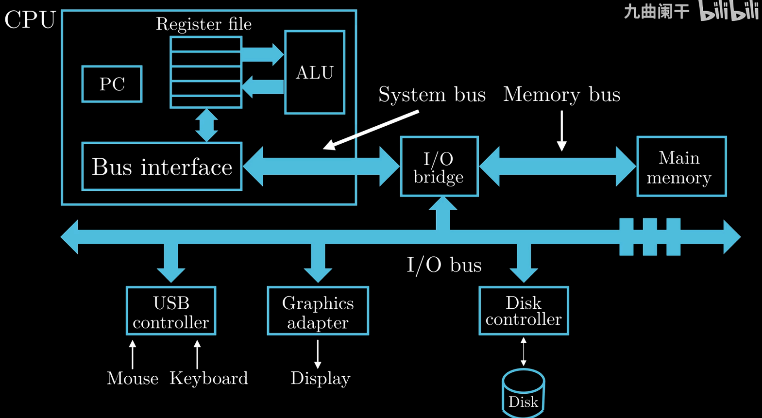
DMA (Direct Memory Access) is usually used for high-spped and bulk data transfers, controlled by system programmers.
-
System Bus
Transfer data in fixed-size blocks called words (4/8 bytes on a 32/64 bit system)
Memory Hierarchy
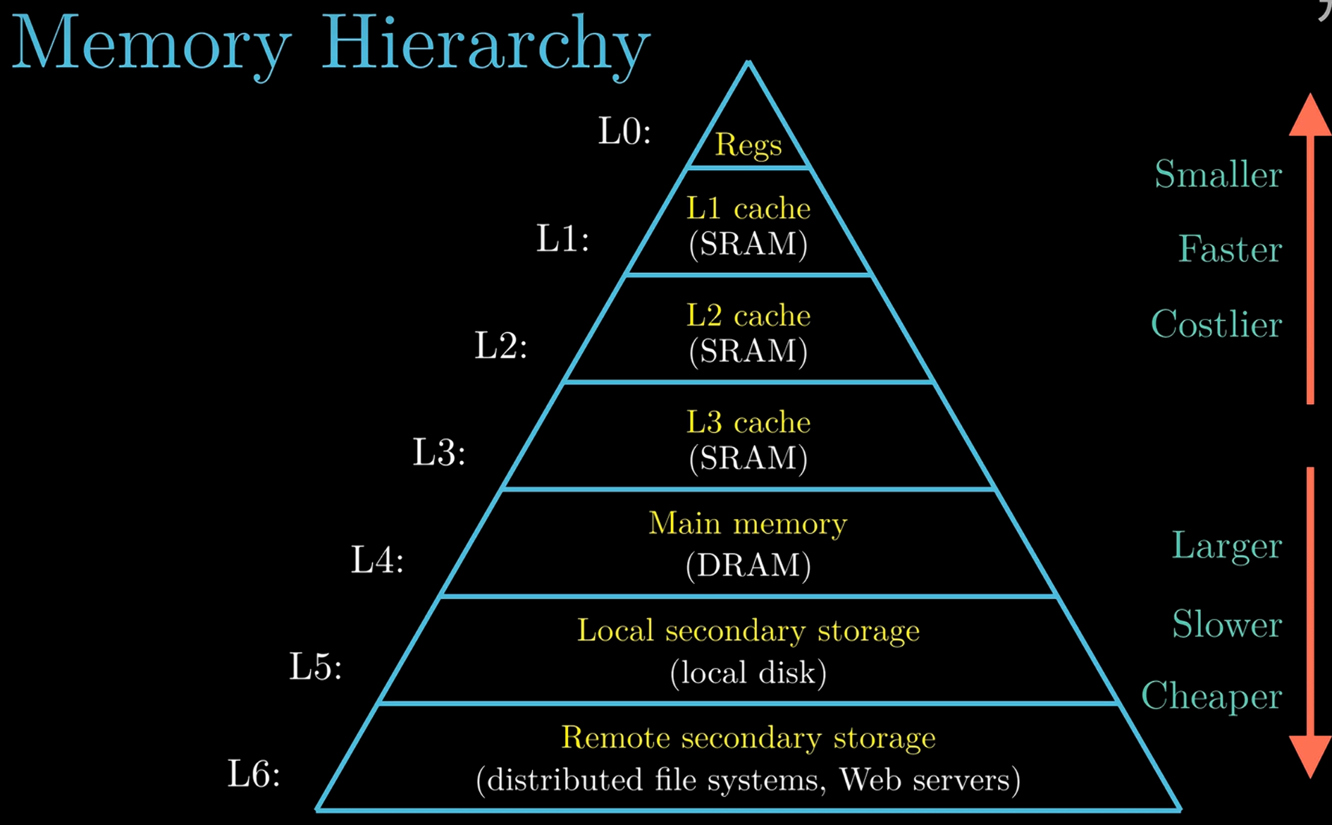
The localities of cache: Temporal Locality & Spatial Locality.
Abstractions in Computer Systems (Virtualization)
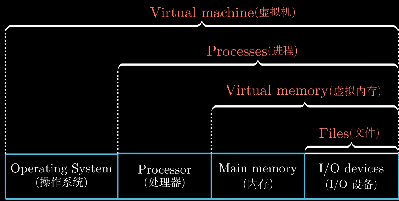
Virtualization is often related to multiplicity, fake versions, and sharing.
-
Process & Thread
Multiple processes can run concurrently on the same system, and each process appears to have exclusive use of the hardware.
Context switching with OS Kernel.
A process can actually consist of multiple execution units, called threads. Threads shares the same code and global data.
-
Virtual Memory
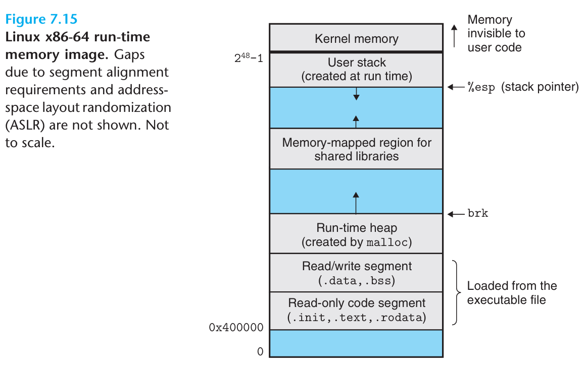
Program Code & Data, Shared Libraries, Heap, Stack, Kernel Virtual Memory from bottom to top.
-
Virtual address space canve greater than the physical memory.
-
Memory serves as a cache for virtaul memory.
-
Support multiprogramming.
-
Allow multiple processes to share data.
-
-
File
Import Themes
Amdahl's Law (Quantifying the performance improvement ceiling)
Concurrency and Parallelism
-
Concurrency It refers to the general concept of a system having multiple, simultaneous activities, which do not necessarily execute at the same time, but may interleave in time to create the logical impression of simultaneity.
-
Parallelism It refers to the use of concureency to make a system run faster.
ILP and DLP
-
Instruction-Level e.g. Parallelism pipelining, superscalar, out-of-order execution.
-
Data-Level Parallelism e.g. Single Insruction Multiple Data (SIMD), Vector instructions.
Computer Architecture
Computer Architecture (e.g. Intel x86, IBM 360, ARM, RISC-V) is the interface between hardware and software, it includes ISA and Microarchitectures (e.g. Different implementations of the same ISA: Single cycle, Multi-cycle, Pipelined, Superscalar, Out-Of-Order, Speculative Execution, Cache Hierarchies, and Various Predictions).
Chapter 2 Representing and Manipulating Information
Information Storage
-
Words
word size virtual address space
-
Addressing and Byte Ordering
Big endian (e.g. IBM Mainframes) & Little endian (e.g. Intel x86, ARM, RISC-V).
Big-endian means most significant byte first, and Little-endian means least significant byte first.
Integer Representaions
Sizes of Data Type in C/C++
| Signed | Unsigned | 32-bit (Bytes) | 64-bit (Bytes) |
|---|---|---|---|
| 1 | 1 | ||
| 2 | 2 | ||
| 4 | 4 | ||
| 4 | 4 | ||
| 8 | 8 | ||
| — | |||
| — | 4 | 4 | |
| — | 8 | 8 |
Unsigned Encodings
Suppose a vector , then
Two's Complement Encodings
Inverse form (1's Complement) For a negative number, keep the signed the same and invert the rest.
two zero exits & end-round carry out issues (hte end carry-out bit needs to add back to the LSB)
2's Complement For a negative number, keep the sign the same, invert the rest and add 1.
Suppose a vector , then
Conversions between Signed and Unsigned
For a -bit 2's complemetn signed binary numeral system:
- Minimum , corresponding to binary (A special case that does not satisfy the invert bits and add 1 rule used for other negative numbers).
- Maximum , corresponding to binary .
Sign Extension
Small to Big
-
Zero extension of unsigned numbers
-
Sign extension of two's complement numbers
Since , by induction, we can proof it.
Big to Small
Integer Arithmetic
Addition
Additive Inverse
-
For two numbers A, B, the overflow occurs when
(NOT (sign_A XOR sign_B)) AND (sign_A XOR new_sign) == 1. (Two operands have the same sign but the result has a different sign.) -
One Bit Full Adder
-
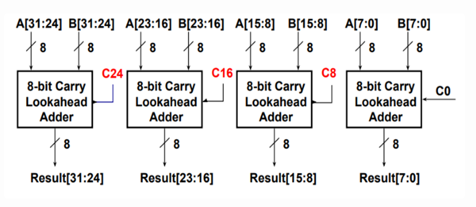
Carry Lookahead Adder
Multipilication
Division (by a power of 2)
Unsigned numbers use logical shift, while two's complement numbers use arithmetic shift to achieve sign-preserving extension.
Right shift performs integer division by powers of two :
Floating Point
Floating-Point Representation
s (sign) : The number is positive () or negative ().
M (fraction) : A binary fraction.
E (exponent) : weight.
()
| Category | Exponent | Fraction | Value Formula |
|---|---|---|---|
| Normalized | any | ||
| Denormalized | |||
| Zero | |||
| Infinity | |||
| NaN (Not a Number) | NaN |
When interpreted as signed integers, the bit representation of IEEE 754 floating-point numbers (excluding NaN) preserves the same sorting order.
Comparison (postive number)
| Format | Minimum | Maximum |
|---|---|---|
| Single Precision Normalized | | |
| Single Precision Denormalized | | |
Rounding
| Round-down | Round-up | Round-toward-zero | Round-to-even |
|---|---|---|---|
Non-midpoint round to the nearest representable value Midpoint choose the one |
Floating Point Operations
-
Lack of Associativity & Lack of Distributivity
Example Questions
Let are of type
int,float,double(Their values are arbitrary, except that neither nor equals , , or .). Then:x == (int)(double) xTruex == (int)(float) xFalse (e.g. )d == (double)(float) dFalse (e.g. )f == (float)(double) fTrued*d >= 0.0True
-
Float Point Addition
- Align decimal points (small to big)
- Add significands
- Normalize
- Round and renormalize if needed
Example
Precision (IEEE 754-2008 Standard Formats)
| Format | Sign Bits | Exponent Bits | Mantissa Bits |
|---|---|---|---|
| Quad precision | 1 | 15 | 112 |
| Double precision | 1 | 11 | 52 |
| Single precision (FP32) | 1 | 8 | 23 |
| Half precision (FP16) | 1 | 5 | 10 |
bfloat16
- The format is 1 sign, 8 exponent, 7 mantissa bits, Same exponent range as FP32.
- AI/LLM is based on predictions, approximation does not require high precision.Therefore reduced precision is acceptable for AI.
- Lower precision format enables higher memory bandwidth and computational. bandwidth.
FMA/FMAC
Fused Multiply and Add (FMA) or Fused Multiply and Accumulate (FMAC) combines multiply and add in one instruction ().
- Multiplication and addition are parallel.
- Normalization and rounding are combined at the end.
Use -mfma -ffp-contract=fast to enable FMA.
Chapter 3 Machine-Level Representation of Programs
Machine-Level Representation of Programs
RISC [optimized for processor speed]
Principles
- Simplicity favors regularity
- Smaller is faster
- Make common cases fast
- Good design demands good compromises
[RSA should be scalable, flexible, and extensible.]
Variants of RV
- RV32, RV64, RV128 Different data widths (addressing capability)
| Extension | Description |
|---|---|
| I | Base integer instructions |
| E | Base for embedded systems (e.g., only 16 registers) |
| M | Integer multiplication and division |
| A | Atomic memory instructions |
| C | Compressed extension (16-bit instructions) |
| F | Single-precision floating point |
| D | Double-precision floating point |
| V | Vector extension |
Instruction Types in RV32I
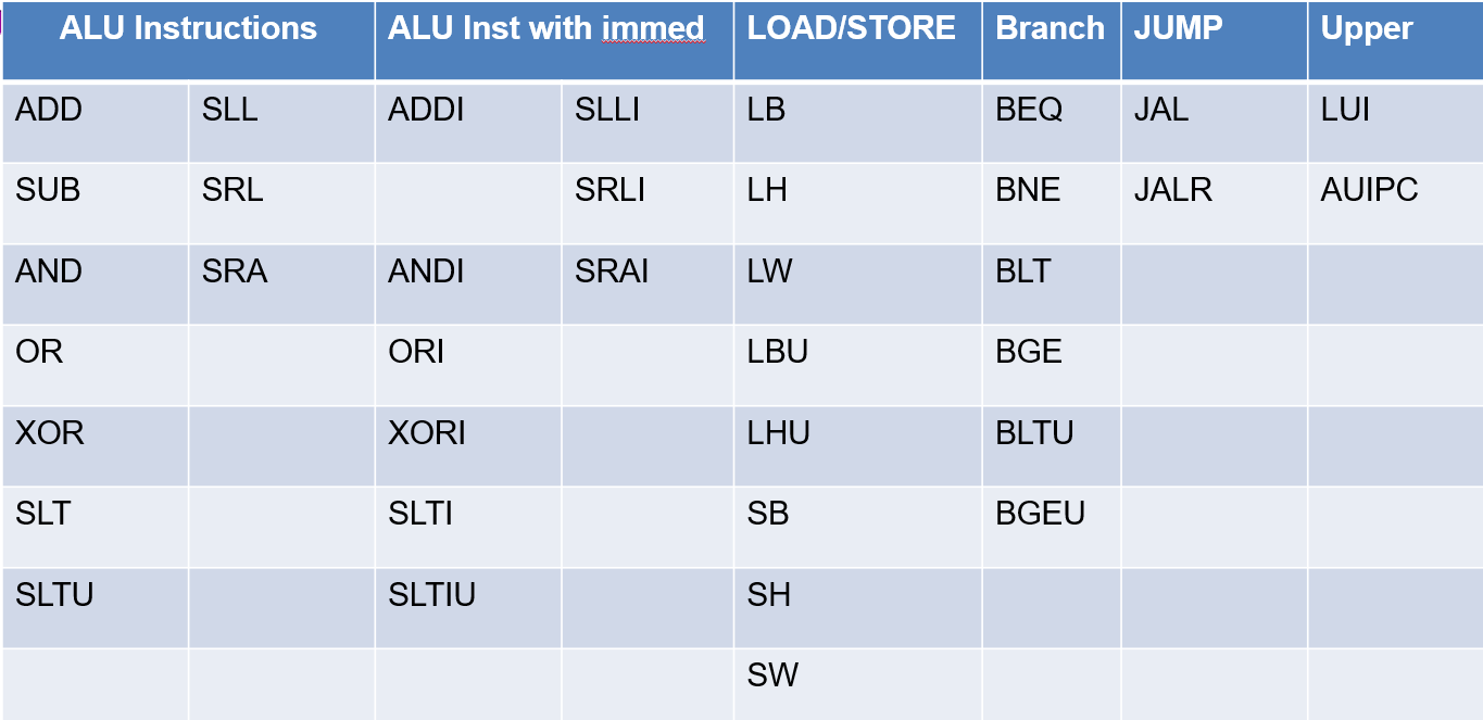
| Types | Instructions |
|---|---|
| ALU | add, sub, and, or, xor, slt, sltu, sll, srl, sra, and all with immediate (No subi in RV32I) |
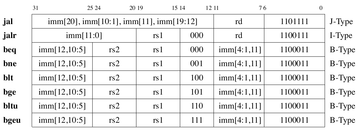
| Control Instructions | beq, bne, blt, bge, bltu, bgeu, jal, jalr |
| Memory Instructions | lw (No lwu in RV32I), lh, lb, sw, sh, sb, lbu, lhu |
| Privileged Instructions | Interrupt, Memory Management, System Calls, Control and Status Registers (CSR), Mode Change |
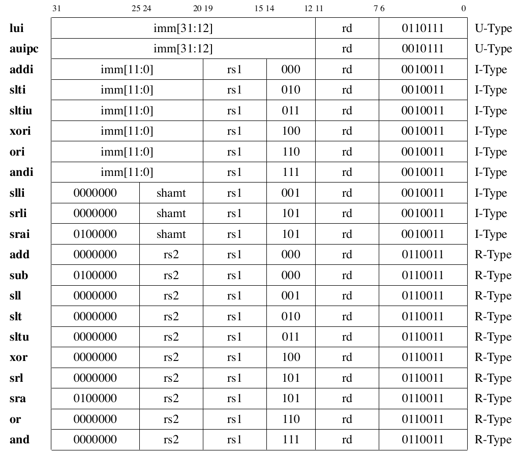
| Format | Name | Instructions |
|---|---|---|
| R-type | Register | add, sub, sll, srl, sra, xor, or, and |
| I-type | Immediate | addi, slli, srli, srai, xori, ori, andi |
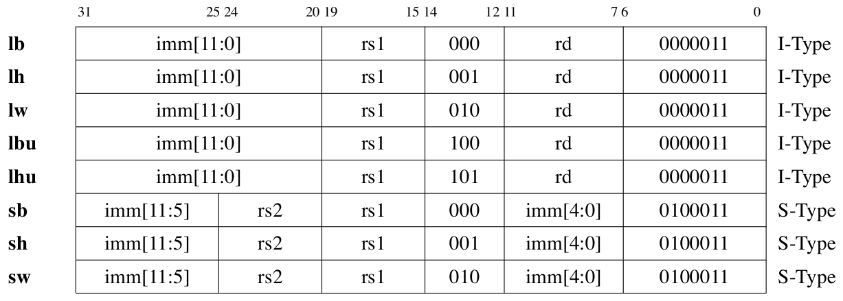
| I-type | Load | lb, lh, lw, lbu, lhu |
| I-type | Jump and Link Register | jalr |
| S-type | Store | sb, sh, sw |
| B-type | Branch | beq, bne, blt, bge, bltu, bgeu |
| U-type | Upper Immediate | lui, auipc |
| UJ-type | Unconditional Jump | jal |
-
Three operand instruction format.
-
X0 is always zero.
-
32 means Address cability/Integer register length.
-
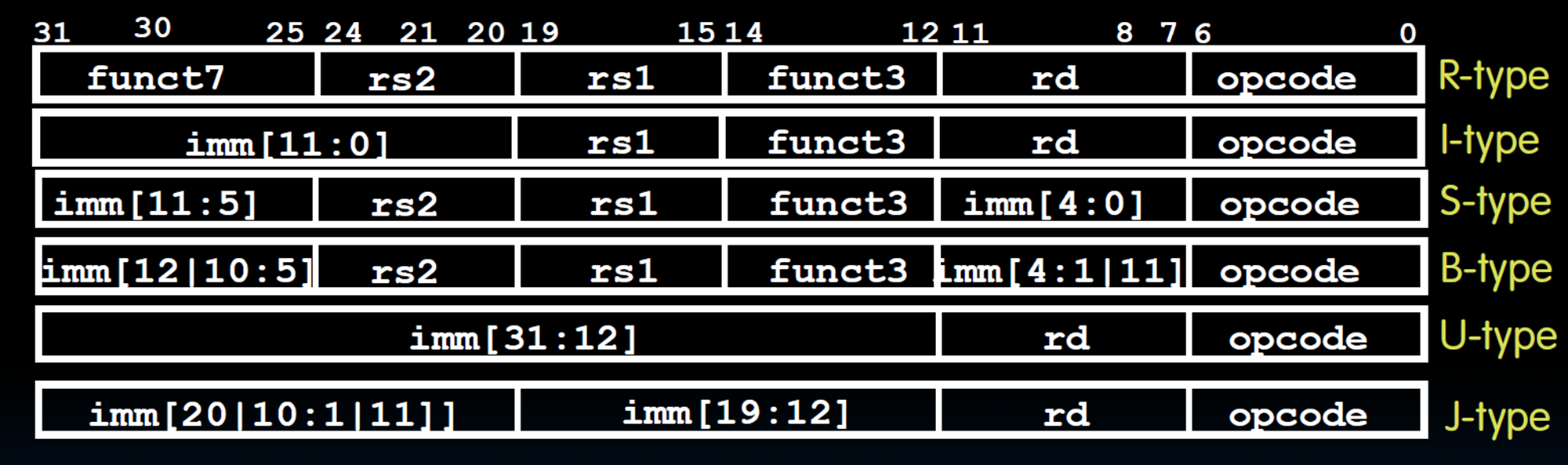
Immediate
- type No immediate.
- type 12 bits immediate. Shift instructions are I-type but repurpose the immediate field as a 5-bit shift amount for RV32I (6-bit for RV64I).
inst[30]distinguishes arithmetic from logical right shift, whileinst[31:26]are fixed to zero exceptinst[30](Range: ). The immediate in the branch instruction is an offset relative to PC. - type The 12‑bit immediate is split into high 7 bits (immediate) and low 5 bits (immed) (maintain regularity). The immediate in the store instruction is an offset relative to
rs1. - type 20 bits immediate.
-
Jump
-
jal- , (Jumps are 2-byte aligned, so last bit is implicit zero).
- Range: .
- Beyond 1MB: Use AUIPC + JALR.
-
jalr- , ( clears LSB to ensure 2‑byte alignment).
-
-
Load and Store
lw rd, offset (rs1)means load data from memory and write intord.sw rs2, offset (rs1)means store data from registerrs2into memory. -
LUI loads a 20‑bit immediate into the upper bits of a register; AUIPC adds a 20‑bit immediate to the current PC for position‑independent addressing.
How to load a 32b const into a register?
- Use a LW instruction (cost more)
luiandaddi(When the lower 12 bits of a 32‑bit constant are ,addisign‑extends them, causing an incorrect result. The assembler automatically adjusts the upper 20 bits when using thelipseudo‑instruction.) (Range: )
Instruction Encoding List
Regularity
| Field | Bit Position | Note |
|---|---|---|
| Opcode | Always opcode | |
| rd | Destination reg | |
| rs1 | Source reg 1 | |
| rs2 | Source reg 2 | |
| Length | - | Fixed 16/32 bit |
| Immediate | High bits | Uses rd field for branch/store |
Pseudo Instrcution
| Pseudoinstruction | Actual Instruction Sequence | Operation |
|---|---|---|
nop | addi x0, x0, 0 | No operation |
li rd, imm | lui rd, imm[31:12] + imm[11]addi rd, rd, imm[11:0] | Load 32-bit immediate |
mv rd, rs | addi rd, rs, 0 | Copy register |
not rd, rs | xori rd, rs, -1 | Bitwise NOT |
neg rd, rs | sub rd, x0, rs | Two's complement negation |
seqz rd, rs | sltiu rd, rs, 1 | Set if |
snez rd, rs | sltu rd, x0, rs | Set if |
sltz rd, rs | slt rd, rs, x0 | Set if |
sgtz rd, rs | slt rd, x0, rs | Set if |
beqz rs, offset | beq rs, x0, offset | Branch if |
bnez rs, offset | bne rs, x0, offset | Branch if |
blez rs, offset | bge x0, rs, offset | Branch if |
bgez rs, offset | bge rs, x0, offset | Branch if |
bltz rs, offset | blt rs, x0, offset | Branch if |
bgtz rs, offset | blt x0, rs, offset | Branch if |
bgt rs, rt, offset | blt rt, rs, offset | Branch if |
ble rs, rt, offset | bge rt, rs, offset | Branch if |
bgtu rs, rt, offset | bltu rt, rs, offset | Branch if unsigned |
bleu rs, rt, offset | bgeu rt, rs, offset | Branch if unsigned |
j offset | jal x0, offset | Unconditional jump |
jal offset | jal x1, offset | Jump and link (return address in x1) |
jr rs | jalr x0, 0(rs) | Jump to address in rs |
jalr rs | jalr x1, 0(rs) | Jump and link to address in rs |
ret | jalr x0, 0(x1) | Return from subroutine |
call offset | auipc x1, offset[31:12] + offset[11]jalr x1, offset[11:0](x1) | Far call to subroutine |
Why do RISC-V loads/stores use base+immediate instead of base+index?
- Simpler hardware Adding scaling to load instructions requires a shifter and complicates the address calculation datapath, increasing cost and cycle time.
- ISA regularity violation Three operands
(rs1, rs2, rd)would force an R‑type format, but R‑type is reserved for ALU operations only. Mixing in memory access would break the clean encoding scheme. - Compiler can optimize it away In loops, the compiler just increments the base register by the element size each iteration, making scaled indexing unnecessary.
Why do RISC-V instructions place immediate bits in seemingly "random" positions (e.g., B-Type and J-Type)?
- Fixed sign bit at position 31 across all formats.
- Decoder reuse (B-Type reuses S-Type logic, J-Type reuses U-Type logic).
- Fixed register fields (
rs1,rs2,rd) across formats.
Application Binary Interface (ABI)
It is based on three key components : the computer ISA, the OS, and the calling convention. ABI incompatibility will occur due to differences between operating systems.
Data Alignment
-
No cache line crossing; no double TLB (Translation Lookaside Buffer) misses; no double page faults come from a single memory instruction execution.
-
Better cache line utilization.
RISC-I to RISC-V do not explicitly enforce data alignments. But their compilers often enforce data alignments.
Crossing a boundary makes the memory reference difficult to handle. The hardware needs to go through two exceptions instead of one.
Padding Rule
- Internal Padding Every member must start at an address that is a multiple of its own alignment requirement.
- Trailing Padding The total size of the struct must be a multiple of the largest alignment requirement among its members.
Exercise
struct S1 {
    int white;
    long long count;
    char c;
    int red;
    int blue;
} A[];
Suppose is an array of structure , and the starting address of is stored in register . what instruction should be used to access A[100].red?
| Member | Size | Start | Padding | End | Reason |
|---|---|---|---|---|---|
white | int aligns at | ||||
count | needs 8-byte align, pad to | ||||
c | char aligns at | ||||
red | needs 4-byte align, pad to | ||||
blue | int aligns at |
Current size is . Largest alignment in struct is , is not a multiple of , so pad bytes at the end. Total struct size is bytes.
A[100].red : , so the answer is LW X2, 3220(X1).
Stack / Frame Alignments
- Defined by ABI (e.g., RISC‑V psABI: 16‑byte)
- CRT aligns
spbeforemain ()
Compiler Reordering
-
Independent Variables (Rearrangement Allowed)
-
Struct Fields (Rearrangement Forbidden)
- Binary compatibility
- Pointer arithmetic
- Interoperability
PC-relative Addressing
Branch instructions use PC‑relative addressing with a 12‑bit signed offset (in 2‑byte units). Since branch targets are always multiples of 2, encoding in 2‑byte units doubles the reachable range without losing information.
CSR
| Name | Abbreviation | Description |
|---|---|---|
| Machine Trap-Vector Base-Address Register | mtvec | Exception handler entry address |
| Machine Status Register | mstatus | Global interrupt enable (MIE) and status |
| Machine Cause Register | mcause | Reason of last exception/interrupt |
| Machine Exception Program Counter | mepc | Saves PC when exception occurs |
| Machine Interrupt Enable Register | mie | Enables specific interrupt sources |
| Machine Interrupt Pending Register | mip | Shows pending interrupts |
Exception Handling
- Save context Save current PC value to
mepcregister - Update status Update
mstatus, disable further interrupts (clear MIE bit) to prevent nesting - Set cause Write exception/interrupt reason to
mcause - Jump to handler Jump to exception handler entry point based on
mtvecconfiguration
Frame Pointer (fp)/Stack Pointer (sp)
- sp points to the top of stack.
- fp points to a fixed location within the current stack frame, typically the address where the old fp is stored.
- When the function returns, the saved old fp is restored to the fp register, making fp point back to the caller's stack frame.
Calling Convention
| RV Registers | ABI Name | Caller/Callee | Purpose |
|---|---|---|---|
| x0 | zero | — | Always zero |
| x1 | ra | Caller | Return address |
| x2 | sp | Callee | Stack pointer |
| x3 | gp | — | Global pointer |
| x4 | tp | — | Thread pointer |
| x5–x7 | t0–t2 | Caller | Temporary registers |
| x8 | s0 / fp | Callee | Saved register / Frame pointer |
| x9 | s1 | Callee | Saved register |
| x10–x11 | a0–a1 | Caller | Arguments / Return values |
| x12–x17 | a2–a7 | Caller | Arguments |
| x18–x27 | s2–s11 | Callee | Saved registers |
| x28–x31 | t3–t6 | Caller | Temporary registers |
- Caller-Saved Caller decides whether to save based on whether the value will be used after the call.
- Callee-Saved Callee must always save these registers before using them and restore them before returning (absolutely safe).
- Array variables are typically allocated in memory (stack or static data section), not in registers.
| Aspect | Caller-Saved | Callee-Saved |
|---|---|---|
| Decision maker | Caller | Callee |
| Mandatory | On demand (only if value is needed after the call) | Yes |
| Save timing | Before calling a subroutine | At function entry |
| Restore timing | After subroutine returns | Before function returns |
Why caller registers are allocated to temporaries?
Temporaries are short-lived and do not need to survive across function calls. Placing them in caller‑save registers avoids unnecessary save/restore code.
Why callee registers are allocated to local variables?
Local variables live across function calls. Using callee registers ensures they are preserved automatically by the callee, avoiding repeated saves at each call site.
Why callee registers are allocated to CSEs (Common Sub-Expressions)?
Local variables and CSEs are tend to live longer (may be as long as the procedure invocation).
CISC [optimized for compact code size]
Chapter 4 Processor Architecture & Logic Design
Logic Designs
Major components
- Combinational element
- State (Sequential) elements , cannot write to register (B-type and S-type).
- Clock signals
What is the difference between combinational logic and sequential logic?
The former one is stateless, output purely depends on the inputs (e.g. ALU). The latter one has states, output depends on the inputs and the states (e.g. register).
The propagation delay of a combinational circuit is determined by the delay of the critical path, which is the longest path of logic gates from any input to any output.
Processor
Core
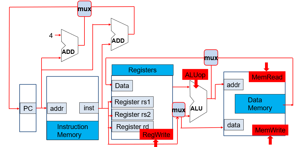
Data Path (Data Flow)
e.g. ALU, Register, Memory interface, Buses.
Control (Instruction Flow)
e.g. PC, Instruction fetch, and Control signal generation.
RV32I Data Path and Control
- Memory reference instrutions
lw,sw - Arithmetic/logical instrutions
add,sub,and,or - Control flow instruction
beq,jal
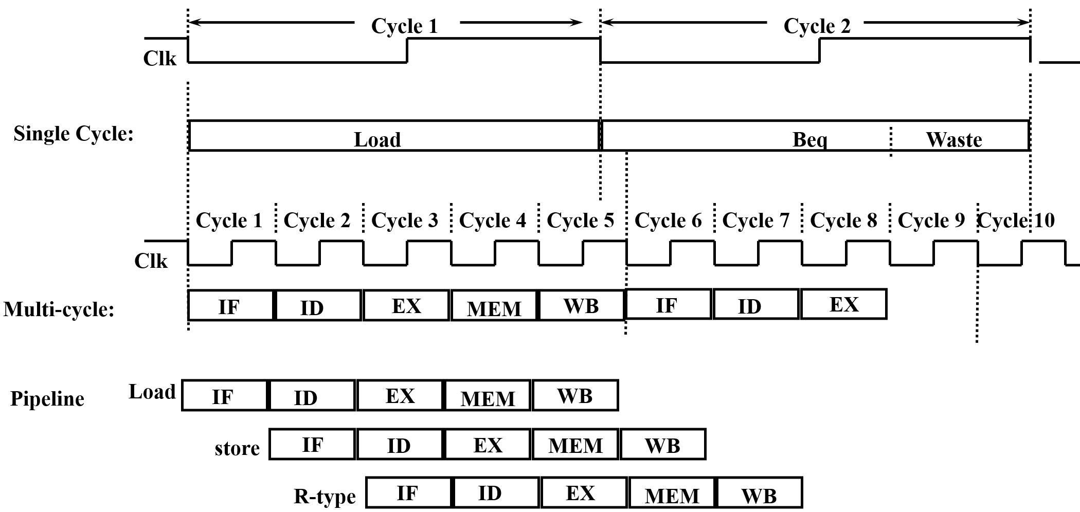
Instruction Execution Cycle
Cycle
-
Three Stages
- Fetch Use the PC to supply the instruction address and fetch the instruction from memory.
- Decode Decode the instruction (and read registers).
- Execute
- Use ALU to calculate (Arithmetic result & Memory address for load/store & branch target address)
- Access data memory for load/store
- Update PC (target address or PC + 4 (next word) or PC + 2 (if using compressed instructions RV32IC))
-
Multi-cycle Instructions are broken down into multiple steps, each taking one clock cycle.
Time
CPU time is determined by the following:
Program execution time is determined by the following:
- CISC machines Lower instruction count, higher CPI, longer cycle time
- RISC machines Higher instruction count, lower CPI, shorter cycle time
Abstract View of RV32I Subset
How to select between PC+4 and PC+immediate?
If a branch is taken or a jal instruction, select pc+immed. Otherwise select PC+4.
Note that jal and jalr use pc + imm as the target address, while writing pc + 4 back to the register. In contrast, auipc writes pc + imm directly back to the register.
How to select data from the memory or the ALU?
If load select Mem. If R-type select ALU.
How to select data from Immediate or reg[rs2]?
If R-type select rs2. If I-type select immed.
Processor Designs
-
Analyze the requirements
-
Data Path Requirements selections
-
Combinational Components Adder & MUX & ALU (An adder only does addition (e.g., PC+4). An ALU includes an adder but also performs many other arithmetic/logic operations.)
-
Sequential Components
Register -bit storage with Write Enable control. Updates only at clock tick if .
Register File consists of 32 registers with two read ports (rs1/rs2) and one write port (rd).
Memory. Read (): Address → Data Out. Write (): Next clock tick, Data In → Address.
-
Assemble
-
Instruction Fetch Unit Fetch the instruction and Update the program counter.
-
Branch Operations Using ALU subtraction for branches risks overflow corrupting the sign, so RISC-V processors internally use flags (overflow and carry) or dedicated comparators for correct branch decisions without hardware traps.
-
Add and Subtract
R[rd] <- R[rs1] op R[rs2] -
Load/Store Operations A single ALU and register file need two multiplexers: one for ALU's second input (e.g.
add rd, rs1, rs2andaddi rd, rs1, imm), another for register file's write data source (e.g.add x3, x1, x2from ALU andlw x3, 8(x1)from memory).
-
-
Control Points and Signals
Control Signal Description Expression PCsrcSelect the next PC value
PC + 4 []
Branch / jump target address [](Branch or jal/jalr) ? 1 : 0RegWrWrite enable for register file (Branch or Store) ? 0 : 1MemRdEnable signal for reading data memory Load ? 1 : 0MemWrEnable signal for writing data memory Store ? 1 : 0ALUsrcSelect the second ALU input
register []
immediate value []R-type ? 0 : 1ALUctrDetermines the ALU operation / WBselSelects the data written to the register file
memory data []
ALU result []
PC + 4 []Load: 0; R-type : 1; jal/jalr : 2
-
On each clock cycle, the single‑cycle processor executes one instruction. State elements update at the rising edge using combinational logic outputs computed during the cycle.
Control
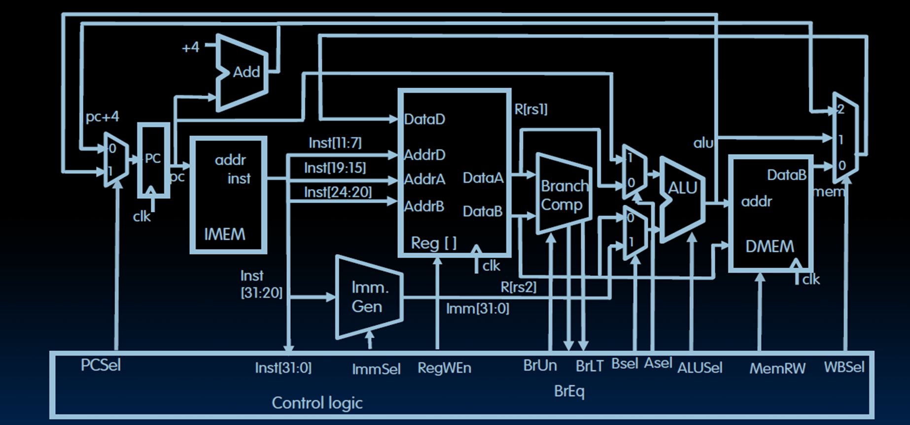
Aselrs1orpc(When usejal, the target isPC + offset.)Bselrs2orimmed.
Why does RV32I still need a dedicated Branch Comparator despite having an ALU?
- Use Branch Comparision to avoid substruction overflow (also faster than subtraction).
- RV32I lacks architectural flags, it requires a dedicated comparator to enable single-cycle compare-and-branch operations by combining comparison and jump logic.
- The ALU at the EXE stage is needed for R-type instructions and Load/Store instructions.
Pipelining
Five Stages
- Instrcution fetch from (instruction) memory
- Instrcution decode & register read
- Execute operation or calculate address
- Access (data) memory operand
- Write the result back to register
| Instructions | Detailed Stages |
|---|---|
R-Type, I-Type, jal, jarl, lui, auipc | (no ) |
| Store, Branch | (no ) |
| Load |
- Throughput increases as more instructions complete per unit time, but single instruction latency (The time it takes for each instruction to be executed.) does not decrease and may even increase.
- Pipeline rate is limited by the slowest stage.
- Potential/ideal speedup = Number of pipeline stages (number of pipeline steps).
- Need to reduce possible fill and drain (e.g., I-cache misses and branch misprediction)
Pipeline-oriented ISA Design
- All instructions are fixed length.
- Few and regular instruction formats.
- Only load/store instructions accessing memory.
- Instructions are simple.
Some principles of designing a pipelined datapath:
- Multi-stage partitioning
- Overlapped execution
- Increased throughput
- Improved resource utilization
Single Cycle & Multi Cycle & Pipeline
| Implementation | Clock Cycle Time | Instruction Latency | CPI |
|---|---|---|---|
| Single-Cycle | Sum of all stage latencies | 1 Clock Cycle Time | |
| Multi-Cycle | Longest stage latency | CPI Clock Cycle Time | |
| Pipelined | Longest stage latency | Number of Stages Clock Cycle Time | (hazards) |
- Latency The total time required to complete one single instruction from start to finish. (Single-cycle data path actually has shorter instruction latency because of the setup time and propagation delay in pipeline.)
- Throughput The total number of instructions completed per unit of time.
- For superscalar implementation, CPI .
- Single cycle as lower throughput but shorter instruction latency.
- No arithmetic exceptions allow out‑of‑order retirement, avoiding stalls for long‑latency instructions.
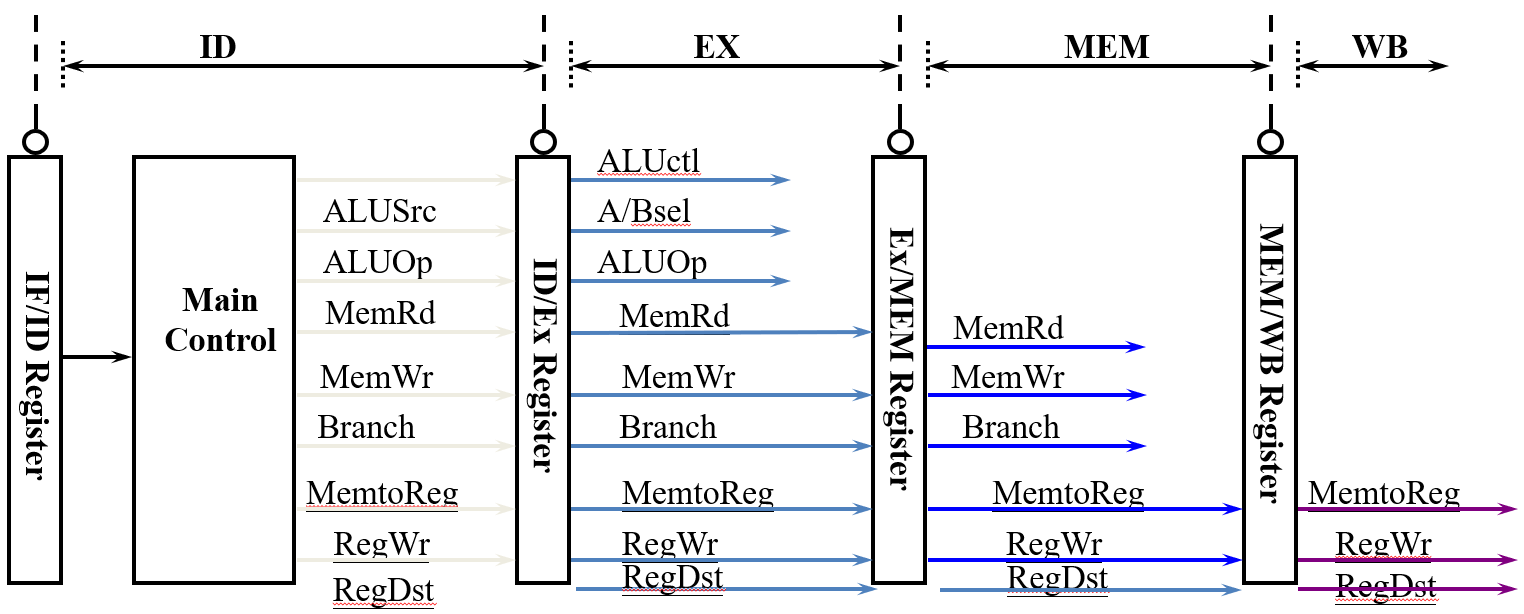
Pipline Registers
Without pipeline registers, stages would overwrite each other’s data, causing instruction mix‑ups and loss of control information.
| Pipeline Register | Stored Information |
|---|---|
| IF/ID | PC_ID, inst_ID (instrcution code like opcode) |
| ID/EX | PC_EX, inst_EX, imm_EX, rs1_EX, rs2_EX |
| EX/MEM | PC_MEM, inst_MEM, rs2_MEM, alu_MEM |
| MEM/WB | PC+4_WB (rd = PC + 4), inst_WB, alu_WB, mem_WB |
-
Control signals are derived from instruction bits, that is, after the ID stage.
-
Control information for later stages are also stored in the pipeline registers.
-
Architecture States (visible to the programmer and compiler)
- Registers (general purpose, fp, vector, flags)
- PC
- Memory
It was saved during a context switch:
- user-level switch (e.g. procedure call) saved on the runtime program stack (caller and callee convention).
- system-level switch (e.g. process switch) saved on the Process Control Block (PCB) or the kernel stack.
-
Micro-architecture states (invisible to the programmer)
- Pipelined registers hold transient data between stages for a few cycles.
- Branch predictors
- Caches
- Buffers and Quenes
- Counters
| Stage | Data Path | Control |
|---|---|---|
rs1, rs2 designators | immed_sel | |
rs1, rs2 contents, PC, immed_value | Asel, Bsel, ALUsel | |
ALUout (Address), rs2 contents | MemRW (read/write), BrLt, Breq | |
ALUout, PC+4 (for link reg), MEMout | Wbsel, rd designator, WRen |
Hazards
Structure Hazards
A conflict arising due to hardware resourece limitations within the pipeline.
-
Pipeline stalls
-
Multiple resources
-
Instruction Reordering
Static scheduling (by compiler) reorders instructions at compile time to avoid hazards, while dynamic scheduling (by hardware) reorders them at runtime based on actual data and resource availability.
-
ISA design
Split Instruction/Data caches can avoid structural hazards in the pipeline and increase the cache access bandwidth.
Data Hazards
A conflict arising because the current instruction depends on the result of a previous instruction that has not yet been computed or written back.
| Scenario | Data Ready Stage | Data Used Stage | Example |
|---|---|---|---|
| Register Access Issues | It bypasses the ALU, read in ID and held until MEM for memory write. | add t0, t1, t2sw t0, 4(t3) | |
| ALU Result Access Issue | add s0, t0, t1 sub t2, s0, t0 | ||
| Load Hazard | lw s1, 4(s0)add t0, s1, t1 |
Solutions
Flow dependence (RAW) is a true data dependence, while anti-dependence (WAR) and output dependence (WAW) are name dependences that can be eliminated by register renaming.
-
Stall pipeline (Interlocking)
-
Data Forwarding (Bypassing)
Add forwarding control logic to make extra connections in the datapath.
Hazard detection compares and destination registers with current instruction’s source registers. (EXE-EXE
EX/MEM.RegRd = ID/EX.RegRs1/2and MEM-EXEMEM/WB.RegRd = ID/EX.RegRs1/2)Forwarding is skipped when
RegWr == 0or when the destination register isx0. -
Compiler Code Transformations
Scheduling (reordering) scope is often limited by branches, indirect branches, and call/ret. Memory aliasing (e.g., and may point to same address) and unknown latencies (e.g. cache hit/miss unpredictable) further restrict reordering. Compiler must conservatively preserve dependencies.
Control Hazards
Control hazards are due to branch instructions (conditional jumps) and JAL/JALR instructions (unconditional jumps).
Condition and Target Address are Ready at the Stage.
Static Branch Prediction (Compile Time)
- Predict a backward branch as taken (loop back branches) and predict a forward branch as fall-through (the compiler always puts the then part in the fall-through path).
- Conditional branch's (e.g.
blt) behavior is entirely program‑dependent and cannot be accurately predicted using simple static rules. Static branch prediction does not read registers at runtime. It only considers whether the branch target is forward or backward. - Unconditional branches (e.g.
jal) always jump, static prediction should always predict taken. - The ISA may reserve a bit in branch instructions as a prediction bit.
- When branch prediction is wrong, pipeline flushing is performed.
Dynamic Branch Prediction (Run Time)
-
Branch History Table (BHT) (Branch prediction should occur at the instruction fetch (IF) stage.)
A branch history table stores past outcomes of branches, indexed by address, to predict future behavior and flush on misprediction.
Tag identifies which address occupies a cache slot. BHT omits tags because prediction bits (1–2) are tiny, tags huge (30–46 bits).
- 1-bit Predictor Flips on every misprediction, fails on nested loops.
- 2-bit Predictor Four-state FSM, changes only after two consecutive mispredictions, handles loops better.
-
Correlated Predictor
Global history register selects a 2-bit counter entry in the pattern table. Current PC selects which table to use, separating histories for different branches.
-
The Location Prediction
Branch Type Prediction Mechanism Example Direct branch Branch Target Buffer (BTB), fixed target beq,jalIndirect branch Hard to predict jalr x0, 4(x1)(Return branch, Switch statements and Function pointers)Function return Return Address Stack (RAS) ret
Chapter 5 Optimizing Program Performance
Compiler Optimization
Compiler Optimization Levels
| Level | Description |
|---|---|
-O0 | No optimizations, fast compile, for debugging. |
-O1 | Basic optimizations. |
-O2 | Recommended default: safe, stable, efficient. |
-O3 | Aggressive (loop unroll, SIMD). May increase code size, compile time, and even hurt performance. |
-O4 | -O3 + Link-Time Optimization (LTO). |
General Goals
Minimize the Number of Instructions
- Common Subexpression Elimination (CSE) Calculate the same expression once and reuse the result.
- Dead Code Elimination (DCE) Don't calculate values that are never used.
- Strength Reduction (SR) Avoid slow instructions (multiplication/division).
Minimize the Execution Cycles
- Register Allocation (RA) Keep frequently used variables in registers.
- Code Scheduling Reorder instructions to avoid stalls.
- Locality Improvement
- Preload & Redundant Load Elimination Load a value once and reuse it, instead of reloading from memory.
Avoid Branching
- Avoid Branching Conditional move in x86 (
cmov, e.g.a = (b > c) ? b : c), conditional execution in ARM (e.g.addgt r0, r1, r2). - Loop Unrolling Reduce the number of branch instructions. Loop unrolling improves performance by reducing the number of branch evaluations and branch mispredictions, also creates opportunities for CSE, code motion, and scheduling.
- Procedure Inlining Reduce the overhead of the call. However, inlining can cause register or I‑cache spilling when code grows too large. For recursive functions, inlining may lead to infinite expansion unless the compiler enforces a depth limit.
- Unswitching Move a condition outside the loop to avoid branching inside the loop. (e.g.
if (cond) { for (...) { ... } } else { for (...) { ... } })
Limitations
-
Compilers cannot change the algorithm.
-
Compilers must obey the rules and semantics of the programming language.
- Memory Aliasing Two pointers may point to the same memory location. Use a local variable for the intermediate value to avoid redundant loads or use the
restrictqualifier to promise no aliasing. - FP Associativity Floating-point addition is not associative.
- Function Side Effects A function may modify global state or have observable effects beyond its return value.
- Volatile Variables A variable declared as
volatilecan be changed by external factors. - Memory Consistency In multi-threaded programs, compilers must respect memory ordering constraints.
- Memory Aliasing Two pointers may point to the same memory location. Use a local variable for the intermediate value to avoid redundant loads or use the
-
Lack of runtime and domain knowledge.
-
Many specific optimization problems are NP-hard.
-
Boundary crossing issues (separate compilation).
Several Optimization Options
| Flag | Description |
|---|---|
-O3 -flto | Link-Time Optimization: enables whole-program optimization. |
-march=native | Generate code optimized for the current CPU architecture (enables all supported instruction sets). |
-mtune=native | Optimize instruction scheduling for the current CPU without breaking compatibility with older CPUs. |
-fprofile-generate | Compile instrumented code to generate runtime profiles. |
-fprofile-use | Use profile data to guide optimizations. |
-Ofast | Alias for -O3 -ffast-math; allows aggressive FP reordering (may break IEEE compliance). |
-fopt-info-missed | Report which optimizations were missed and why. |
Chapter 6 The Memory Hierarchy
Storage Technologies
Access time is the same for all locations.
All unconventional DRAM chips offer much higher bandwidth, but the latency remains the same (The first data still takes the same time to arrive).
| Feature | SRAM | DRAM |
|---|---|---|
| Transistors per bit | ||
| Access time | 1× | 10× |
| Refresh | No | Yes |
| Error Detection and Correction | Optional | Yes |
| Cost | High | Low |
| Main applications | cache memories | main memory, frame buffers |
Static Random Access Memory (SRAM)
Dynamic Random Access Memory (DRAM)
- Reading DRAM Supercell Select row via RAS, load into buffer. Select column via CAS, output data, then rewrite row to refresh.
- Memory Modules A 64-bit word is stored across eight DRAM chips in parallel, with each chip providing one byte (8 bits) at the same row and column address.
Memory Wall
The gap between the speed of processors and the main memory. The bottleneck has shifted from how fast memory can respond (latency) to how much data it can deliver per second (bandwidth).
Latency
- Reduction local memory, NUMA, PIM (Reduce the waiting time for each visit.)
- Hiding multi-threading/Hyper-threading, WARP interleaving, chip-multithreading (Keep computation units busy.)
Bandwidth
- Memory bandwidth multi-banks and interleaved memory, SDRAM, HBM
- Communication bandwith wider bus, interconnection network
Locality
Principle
Many Programs tend to use data and instructions with addresses near or equal to those they have used recently.
emporal locality
Recently referenced items are likely to be referenced again in the near future.
Spatial locality
Items with nearby addresses tend to be referenced close together in time.
What locality is exhibited by the following C loop?
while (A != NULL) A = A->next;
A. Data temporal locality B. Data spatial locality C. Structural locality D. Instruction temporal locality E. Instruction spatial locality
Answer
D and E. The loop repeatedly executes the same small set of contiguous instructions (instruction spatial locality) and reuses those instruction addresses across iterations (instruction temporal locality); data locality is absent because each list node is accessed only once and nodes may not be contiguous in memory.
Memory Hierarchy
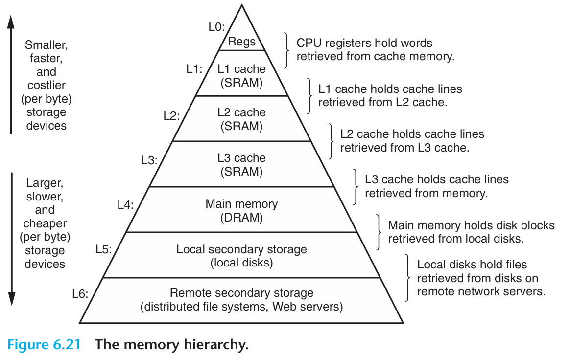
| Level Transfer | Staging Unit | Typical Size | Controlled By |
|---|---|---|---|
| Registers ↔ Memory | Instruction Operands | Bits / words (e.g., 32/64 bits) | Compiler (Programmer) |
| Cache / Local Memory ↔ Memory | Blocks / Lines | 64 B (cache line) | Hardware (Cache Controller) / Compiler or Programmer (Local Memory) |
| Memory ↔ Disks | Pages | 4 KB (page) | Hardware & OS (Virtual Memory) / Programmer (Files) |
| Disks ↔ Tapes | Files | Variable (e.g., 64 KB–1 MB) | Hardware / Operator or Programmer |
This gives you Large, Cheap memory, but Fast access.
Caches provide automatic (transparent) data movement, while local memory requires explicit programmer-controlled data management.
Cache Management
General Cache Memory Organization
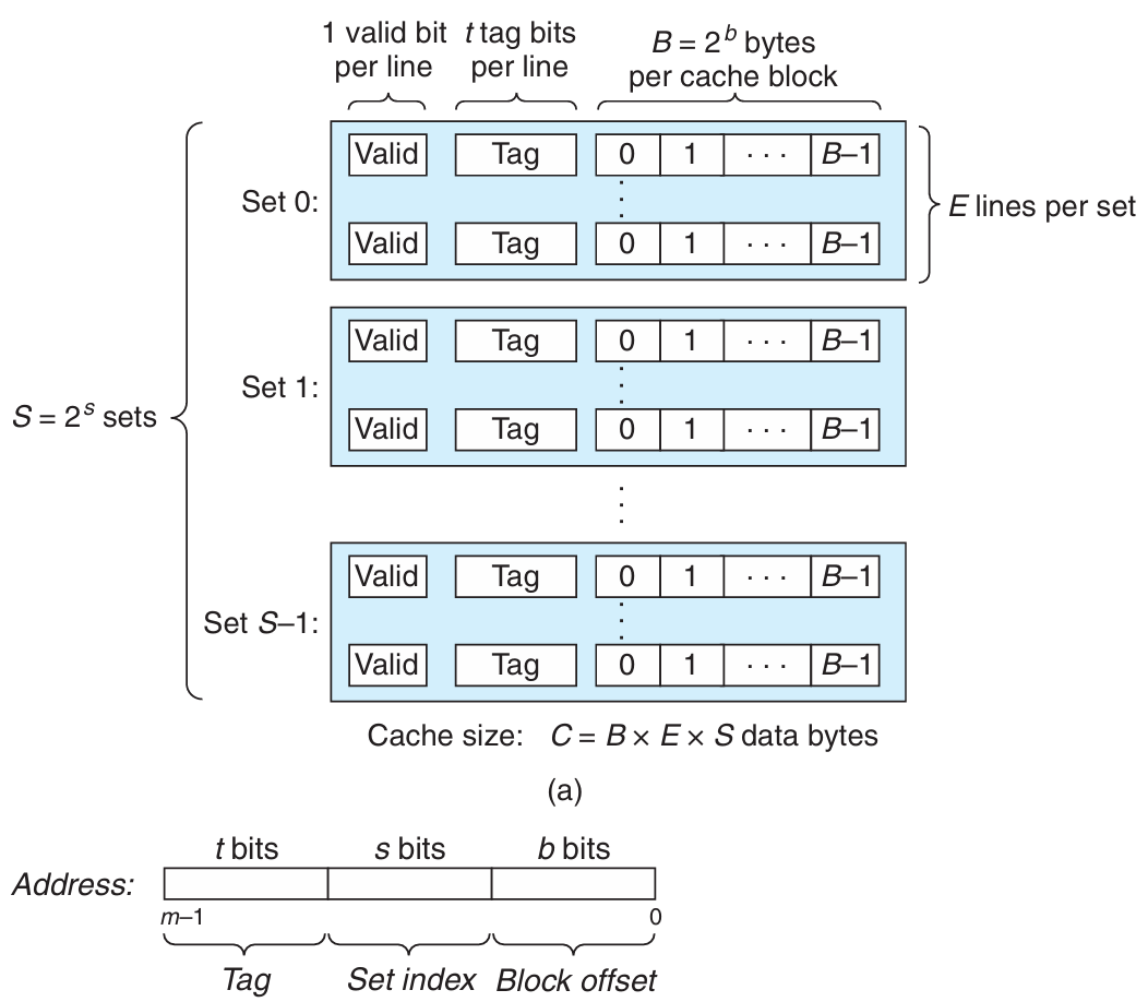
Direct Mapped Caches
-
Valid Bit
A cache line is invalid (valid bit equals to ) when:
- When a cache line of data has not come back from memory yet
- Cache line is currently being replaced
- Cache is flushed
-
Three Steps
- Set Selection Use the set index as an unsigned binary number to locate the cache set.
- Line Matching Compare the tag to determine if the desired block is present in the set.
- Word Extraction Use the block offset as a binary number to select the appropriate word within the cache line.
Why is the set index typically taken from the middle bits of the address rather than the high bits?
Using high bits as the set index causes consecutive memory blocks to map to the same set, leading to more conflict misses, whereas middle bits distribute blocks across sets to better exploit spatial locality.
Set Associative Caches
-way set-associative has lines per set while direct-mapped is one way and fully associative is one set.
Given a cache with total size measured in kilobytes, associativity , and block size measured in bytes. The number of sets is calculated as .
Performance Impact of Cache Parameters
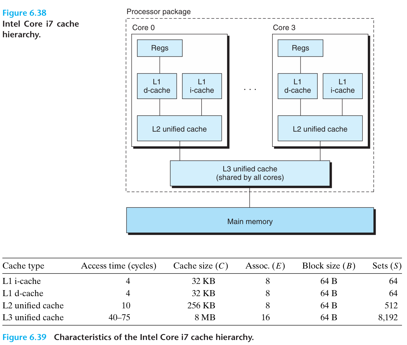
| Feature | L1 Cache | L2 Cache |
|---|---|---|
| Primary goal | Minimize hit time | Minimize miss rate |
| Locality preference | Spatial locality | Temporal locality |
| Typical write policy | Write-through | Write-back |
| Reason | L1 hit directly affects pipeline | L2 miss leads to high memory penalty |
| Associativity | Low | High |
| Size | Small | Large |
- When the block size is too small, the cache cannot fetch enough contiguous data in a single miss (lower spatial locality -- most accesses to nearby addresses still result in cache misses).
- When the block size is too large, the fixed-size cache holds fewer blocks, leading to more conflicts, frequent replacements and higher miss penalty (lower temporal locality -- the recently used data is quickly evicted before it can be reused).
- Number of cache lines is determined by the cache size and the line size.
| Parameter / Change | Block Offset Bits | Set Index Bits | Tag Bits |
|---|---|---|---|
| Formula (64‑bit address) | |||
| Increase block size | — | ||
| Increase cache size | — | ||
| Increase associativity | — |
Cache Hit and Miss
Cache Read
-
Read Hit
-
Read Miss When a read miss occurs, the CPU stalls the pipeline, fetches the missing block from the next memory level, and then resumes execution.
Cache Write
-
Write Hit
-
Write Through
It simultaneously updated to cache and memory. It ensures data isn't lost if the cache is disrupted, but increases memory traffic and write latency.
Solution: write buffer. A write buffer hides write latency, but if store frequency exceeds the DRAM write cycle, the buffer saturates and stalls the CPU (Write buffer allows write-coalescing/combining to reduce traffic to memory.).
-
Write Back
The CPU writes data only to the cache initially, and main memory is not updated until the cache line is eventually replaced (need Dirty Bit). This reduces memory traffic and write latency, but creates cache-memory inconsistency, requiring cache coherence protocols (e.g., MESI) in multi-core systems. Data loss risk on cache failure is mitigated by Error Correcting Code (ECC) protection.
-
-
Write Miss
- Write Allocate First read the data from main memory and loaded into the cache, and then the write operation is performed on the cached copy.
- No Write Allocate It writes the data directly to main memory without loading the missing block into the cache (Better for streaming writes, e.g. writing database logs).
| Aspect | Write Through + No Write Allocate | Write Back + Write Allocate |
|---|---|---|
| Write Miss Behavior | Bypass cache, write directly to main memory (optionally via write buffer + write-combining) | Load missing block from main memory into cache first, then write to cache |
| Typical Partner | Write Through Cache | Copy Back (Write Back) Cache |
| Initial Cost | Low (no main memory read) | High (one read miss) |
| Reuse Cost | High (data not in cache, still miss on reuse) | Low (subsequent reads/writes hit in cache, only set dirty bit) |
| Best For | Write once, never reused data (e.g., writing logs) | Repeated reads/writes to same data (temporal locality) |
Instruction Cache Miss Handling
On an instruction cache miss, the CPU sends the PC to memory, waits for the read to complete, writes the fetched data into cache with its tag and valid bit set, then restarts the instruction fetch. (Instruction cache prefetching is a commonly used hardware optimization to reduce instruction cache misses.)
Can you prefetch for instruction cache in software?
Software cannot directly prefetch instructions (the fetch stage is PC-driven), unlike data prefetching. It can only indirectly affect I-cache hit rate via code layout or execution order.
If we prefetch on every miss, why not just use a larger cache line size?
- Branch-sensitive Prefetching follows the predicted path, fetching only useful instructions. Large lines load all adjacent instructions regardless of branches, wasting bandwidth and cache space on dead code.
- False sharing Large lines reduce effective cache capacity, more likely to cause conflict.
- Bandwidth-aware Large line increases the cost of every miss. Prefetch is more flexible.
Why does the GPU prefetch for the next 10-12 lines, but the CPU only prefetches for 1-2 lines?
GPU prefetches 10–12 lines because it is throughput‑oriented with highly linear instruction flow, making deep prefetch safe, while CPU, being latency‑sensitive with frequent branches, only prefetches 1–2 lines to avoid polluting the cache and wasting bandwidth on wrong paths.
Types of Cache Misses
- Compulsory (or Cold) Miss The first access to a block that has never been loaded into the cache before. (Hardware prefetching & larger cache line size to reduce compulsory misses.)
- Conflict (or Collision) Miss Multiple references are mapping to the same set, and the set is not large enough to hold them.
- Capacity Miss Cache is not large enough to hold needed blocks.
- Coherence Miss Caused by invalidation from other processors in a multiprocessor system to maintain cache coherence.
Ways to Reduce Cache Miss Penalty
| Technique | Core Idea | How It Hides Penalty |
|---|---|---|
| Critical Word First and Early Restart | Fetch requested word first; resume execution immediately | Reduces wait time; overlaps load with execution |
| Non-Blocking Cache | Continue on miss; track multiple misses with MSHRs | Overlaps multiple misses |
| Cache Prefetching | Fetch data before it is needed | Avoids miss entirely |
| Write Buffer | Hold dirty blocks temporarily; write back later | CPU doesn't wait for write |
| Cache-Aware Code Scheduling | Compiler reorders instructions | Overlaps miss with computation |
Non-Blocking Cache and Blocking Cache
Blocking Cache
A cache miss stalls the CPU pipeline immediately (stall on miss).
Non-Blocking Cache (Lockup-Free Cache)
The CPU continues executing other instructions on a miss and stalls only when the data is needed, using Miss Status Holding Register (MSHRs) to track outstanding misses (stall on use). Non-blocking caches support MLP (Memory Level Parallelism).
- Hit under Miss During one miss, the cache can still handle subsequent hits.
- Miss under Miss (better) During one miss, the cache can also handle another miss, allowing multiple outstanding misses.
Cache Block Replacement
Direct Mapped
Each set has only one line, so the new block always replaces the existing block in that set.
Set ssociative or Fully Associative
-
Random
-
Least Recently Used (LRU) [stack algorithm]
Hardware keeps track of the access history and replaces the block that has not been used for the longest time.
Each block has a counter. On a hit, reset its counter to 0 and increment all other counters in the set. On a miss, replace the block with the highest counter value.
-
First In First Out (FIFO) The block that has been in the cache the longest is replaced, regardless of access history.
-
Belady’s Algorithm [upper bound]
Replace the block that will not be used for the longest time in the future. It is optimal but requires perfect knowledge of future accesses, making it impractical for real hardware.
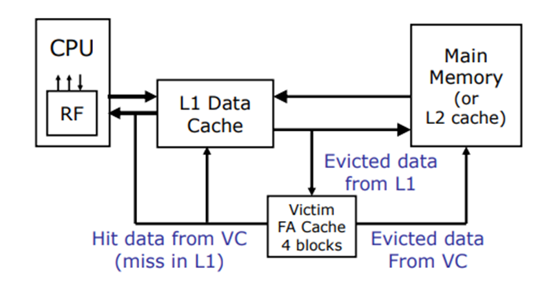
Victim Cache
A small fully associative cache placed between the main cache and memory to hold recently evicted blocks, reducing conflict misses by providing a second chance for recently replaced data. Since such conflicts occur in only a few sets, just 4–8 entries suffice for fast access, combining the speed of direct-mapped L1 with the benefit of full associativity.
Snoopy Cache Coherence Schemes
Snoopy cache maintains coherence in bus-connected multi-processors by broadcasting all coherence operations over a shared bus. Every cache controller snoops the bus and reacts based on its local cache state. Each controller is a bidirectional state machine that processes CPU requests and bus snoop events, updating states according to a transition diagram.
Multiple controllers form a distributed algorithm operating at cache block granularity. The MESI protocol, with its four states (Modified, Exclusive, Shared, Invalid), tracks each block to enable coherence while minimizing bus traffic and memory accesses.
Exclusive/Inclusive Caches
Inclusive L2 caches simplify coherence invalidation in multiprocessor systems by checking at the L2 level, despite wasting capacity, which modern processors tolerate for easier consistency management, making inclusive more common than exclusive today.
Inclusive caches
Every line in L1 must be presented in L2 (). When L2 evicts a line, it must invalidate the corresponding line in L1, and L2 can have a larger line size than L1.
Exclusive caches
If a line, A, is in L1, it must NOT be presented in L2. AMD had adopted this for L2/L3. When L1 evicts a line, it moves to L2. On an L1 miss that hits in L2, the line migrates from L2 to L1. And L1 and L2 must have the same line size.
NINE (Non-Inclusive and Non-Exclusive)
More suitable for L2/L3.
Average Memory Access Time (AMAT)
Usually, %instr is higher than %data, but I-cache hits better because instruction accesses are highly sequential with strong spatial locality, have no write misses (read-only), and exhibit simpler access patterns than data references, which often involve random pointers or strided array accesses.
AMAT was accurate for blocking caches and in-order CPUs, but lost relevance as out-of-order execution, non-blocking caches, prefetching hid miss latency and spliting I/D caches.
Low Hit Latency
- Small and Simple
- Direct-map or low associativity Number of comparators needed equals total cache entries for fully associative, but only for -way set associative.
- Prediction Predict which way to compare first.
- Virtual address cache or virtual index and physical tagged cache Avoid or overlap with address translation delay.
- Cache layout closer to CPU to minimize signal delay
Chapter 7 Linking
Why Linking Matters
Modularity
Separate compilation allows developers to work on different modules independently, improving productivity and enabling code reuse.
Efficiency
- Time Separate compilation & Parallel compilation.
- Space Static linking (Executable files and running memory images contain only the library code they actually use.) & Dynamic linking (Executable files contain no library code. During execution, a single copy of the library code is shared among all executing processes.)
Static Linking
Symbol Resolution
Symbol tables in object files record symbol definitions (name, size, location), and the linker matches each symbol reference to exactly one definition during symbol resolution.
Link Symbols
| Type | Description | Example |
|---|---|---|
| Global symbols | Defined by module m, can be referenced by other modules. | int global_var = 10;void func() { } |
| External symbols | Referenced by module m but defined by some other module. | extern int global_var;extern void func(); |
| Local symbols | Defined and referenced exclusively by module m. | static int local_var = 10;static void helper() { } |
Strong symbols are procedures and initialized globals, while weak symbols are uninitialized globals. Linker's Symbol Rules: Multiple strong symbols are forbidden; one strong wins over weak; multiple weak are arbitrary, unless -fno-common forces an error.
Example
-
file1.cint x = 10; // strong symbol int y = 5; // strong symbol void p1() {printf("x = %d, y = %d\n", x, y);} -
file2.cdouble x; // weak symbol void p2() {printf("x = %f\n", x);}
Writes to in p2 might overwrite .
Avoid global symbols if possible, otherwise use static to limit scope, initialize globals to make them strong, and reference external globals with extern to avoid linker errors.
Static Libraries
Concatenate related relocatable object files into a single file with an index (called an archive). For example, ar rs libfoo.a a.o b.o c.o creates a static library libfoo.a containing a.o, b.o, and c.o.
Linkers scan files left to right, maintain an unresolved reference list, and only extract archive members that resolve current entries, so libraries must come at the end of the command line.
The solution to deal with the order sensitivity and duplicate symbol definitions is to introduce Shared libraries are object files whose code and data are loaded and linked into an application dynamically, either at load time or at run time.
Relocation
It first merges all separate code and data sections into single sections. Then, it relocates symbols from their relative offsets in .o files to final absolute addresses in the executable. Finally, it updates every reference to these symbols to reflect their new positions.
Object Files
Classification
| Type | Extension (Linux/Unix) | Description |
|---|---|---|
| Relocatable Object File | .o | Contains code and data in a form that can be combined with other relocatable object files to form an executable object file. Each .o file is produced from exactly one source (.c) file. |
| Executable Object File | a.out | Contains code and data in a form that can be copied directly into memory and then executed. |
| Shared Object File | .so | Special type of relocatable object file that can be loaded into memory and linked dynamically, at either load time or run-time. It also called Dynamic Link Libraries (DLLs) by Windows. |
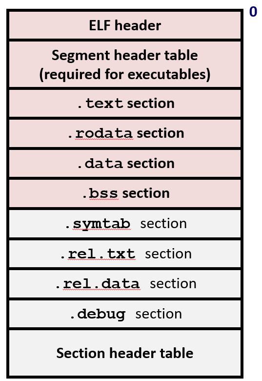
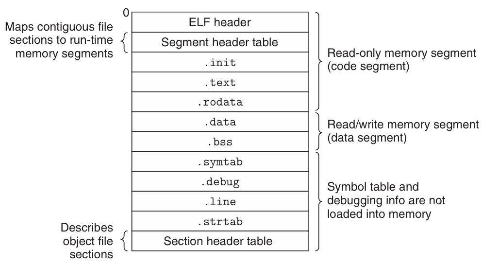
ELF Object File Format
| Component | Description |
|---|---|
| ELF Header | Word size, byte ordering, file type (.o / executable / .so), machine type, etc. |
| Segment Header Table (for OS) | Page size, virtual address memory segments (sections), segment sizes. |
| .text | Code |
| .rodata | Read-only data: jump tables, string constants, etc. |
| .data | Initialized global variables and initialized local static variables. |
| .bss | Uninitialized global variables and uninitialized local static variables. Has section header but occupies no space. |
| .symtab | Symbol table: procedure names, global variable names, static variable names, external symbols, section names, and their locations. |
| .rel.text | Relocation info for .text section: addresses of instructions that will need to be modified in the executable, plus instructions for modifying. |
| .rel.data | Relocation info for .data section: addresses of pointer data that will need to be modified in the merged executable. |
| .debug | Info for symbolic debugging (generated with gcc -g). |
| Section Header Table (for execution and debugging) | Offsets and sizes of each section. |
-
Using the command
readelf -s <file>to view the symbol table of an Executable and Linkable Format (ELF) file. -
Note that Local non-static variables are stored on the stack.
-
It will create local symbols in the symbol table with unique names.
Executable Object Files
Load Executable Object Files
Dynamic Linking with Shared Libraries
Load-Time Linking
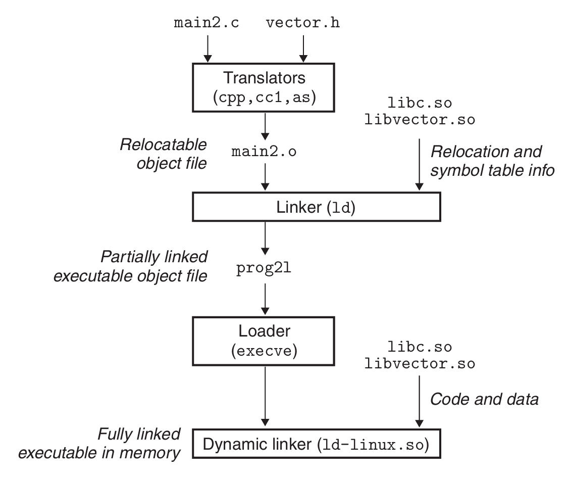
It occurs when the executable is first loaded and run. The standard C library (libc.so) is typically dynamically linked this way.
LD_PRELOAD forces the dynamic linker to load a user-specified shared library first, allowing interception of standard functions, but cannot intercept statically linked _start.
Run-Time Linking
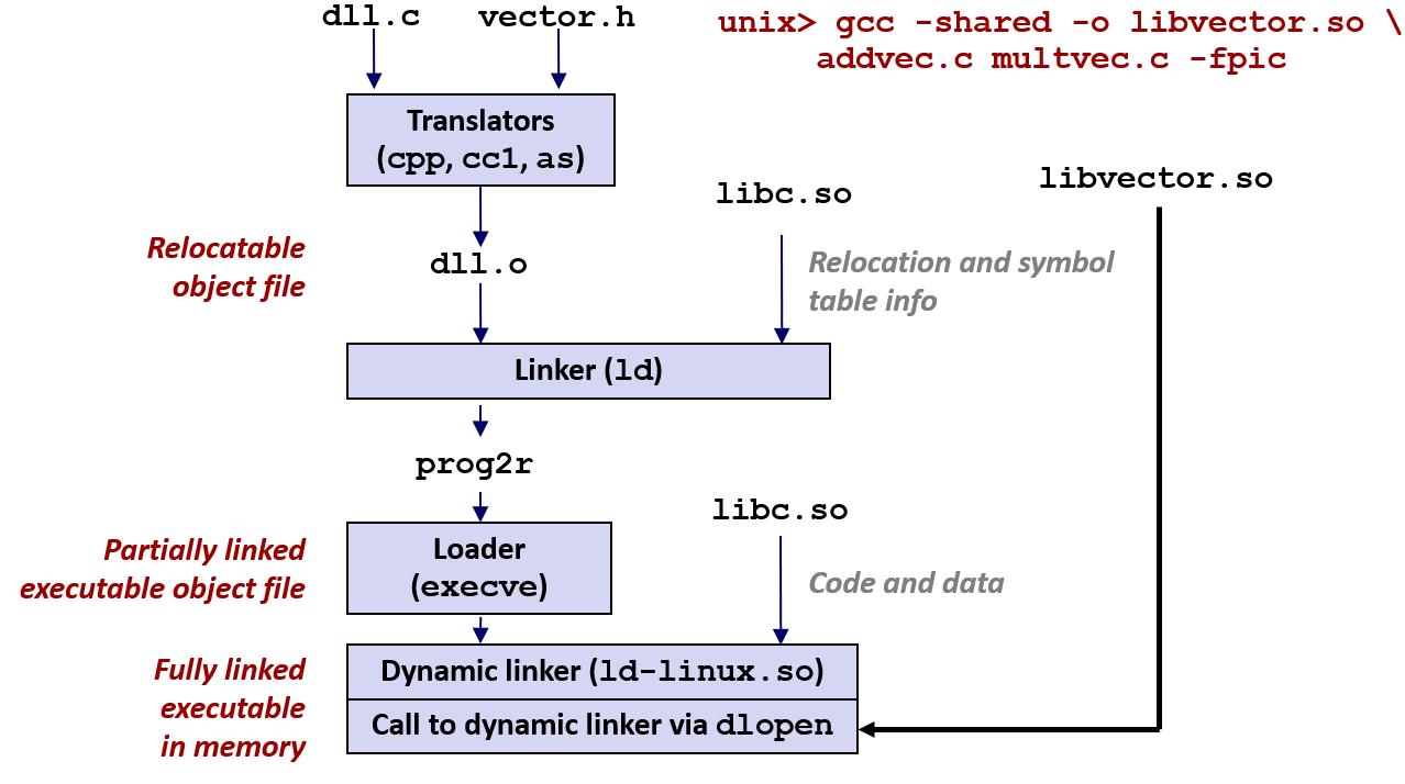
It occurs after the program has begun, using calls to the dlopen() interface on Linux.
Position-Independent Code (PIC)
To exploit the fact that the distance between any instruction in the code segment and any variable in the data segment is a runtime constant, the compiler creates a table called the Global Offset Table (GOT) that holds the absolute addresses of global variables.
Global Offset Table (GOT)
Resides in the data segment and stores the actual absolute addresses of external functions and global variables. These addresses are filled in by the dynamic linker at load time or on the first call.
Procedure Linkage Table (PLT)
A memory section containing small executable stubs for each external function the program calls. It lives in a read-only code section (.text or .plt), providing a trampoline that jumps through the GOT to the actual function.
.got stores addresses of global variables for direct access, while .got.plt stores addresses of external functions specifically for PLT stubs
Whole Process
| Step | Stage | Action |
|---|---|---|
| 1 | Compile (static time) | Compiler generates pseudo instruction: call printf |
| 2 | Compile (static time) | Assembler expands to auipc+jalr, adds reloc entries |
| 3 | Link (walk time) | Linker creates .plt stub (auipc+ld+jalr) |
| 4 | Link (walk time) | Linker allocates GOT entry (44B for 32b, 8B for 64b) |
| 5 | Dynamic Linking (run time) | Dynamic linker fills GOT with real printf address |
Chapter3
CISC [optimized for compact code size]
Size of Data Type in IA32
| C declaration | Intel data type | Assembly-code suffix | Size (bytes) |
|---|---|---|---|
| Byte | |||
| Word | |||
| Double word | |||
| Quad word | |||
| Quad word | |||
| Single precision | |||
| Double precision |
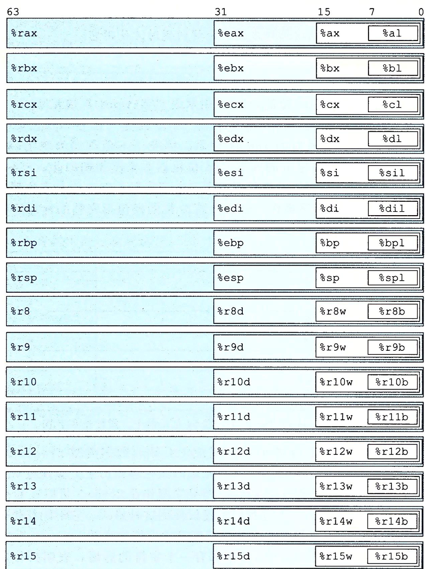
Register
Operands
-
Immediate
-
Register
-
Memory Reference Immediate & Base Register & Index Register & Scale Factor (1,2,4,8)
| Type | Form | Operator Value | Name |
|---|---|---|---|
| Immediate | Immediate | ||
| Register | Register | ||
| Memory | Scaled Indexed | ||
| Memory | Absolute | ||
| Memory | Indirect | ||
| Memory | Base + Displacement | ||
| Memory | Indexed | ||
| Memory | Indexed | ||
| Memory | Scale Indexed | ||
| Memory | Scale Indexed | ||
| Memory | Scale Indexed |
Operation code
-
Movement
-
[
movb,movw,movl,movq,movabsq]Source operand (Immedita, Register, Memory); Destination operand (Register, Memory)
Two operands of a move instruction cannot both be memory references. (It is necessary to first move the source memory reference into a register, and then move it to the destination memory reference.)
movlwrites 32 bits of data to the lower half and then automatically zero-extends the value into the upper 32 bits. (In x86-64, any instruction that generates a 32-bit result for a register will set the upper 32 bits of that register to zero.)movqcan only be 32 bits (sign-extended to 64 bits), whereasmovabsqcan be 64-bit but the destination must be a register. -
[
movzbw,movzbl,movzwl,movzbq,movzwq]movzlqdoes not exist because ofmovlinstruction. -
[
movsbw,movsbl,movswl,movsbq,movswq,movslq,cltq]cltqsame asmovslq %eax, %rax
-
-
Stack
let a quad number be the example
-
subq $8 %rsp movq %rbq,(%rsp) -
movq (%rsq),%rax
addq $8, %rsp
-
Load Effective Address
Computes effective address and stores it in destination register
Unary Operations
| Instructions | Effect |
|---|---|
inc D | |
dec D | |
neg D | |
not D |
Binary Operations
| Instructions | Effect |
|---|---|
add S D | |
sub S D | |
imul S D | |
xor S D | |
or S D | |
and S D |
Shift Operations
| Instructions | Effect |
|---|---|
sal D | |
shl D | |
sar D | Arithmetic Right Shift |
shr D | Logical Right Shift |
Shift instructions can shift by an immediate value, or by a value placed in the single-byte register %cl.
Condition Code
-
Carry Flag [check for overflow in unsigned operations]
-
Zero Flag
-
Sign Flag
-
Overflow Flag
-
Similar to
sub, but it only sets the condition codes without changing the value of the destination register.When
S == D, .It will set the condition codes based on the result of .
-
Similar to
and, but it only sets the condition codes without changing the value of the destination register.When
S & D == 0, .
Set Instructions
| Instruction | Effect | Description |
|---|---|---|
sete D | ||
setne D | ||
sets D | negative | |
setns D | nonnegative | |
setg D | Signed | |
setge D | Signed | |
setl D | Signed | |
setle D | Signed | |
seta D | Unsigned | |
setae D | Unsigned | |
setb D | Unsigned | |
setbe D | Unsigned |
Jump Instructions
| Instruction | Jump Condition | Description |
|---|---|---|
jmp Label | Direct Jump | |
jmp *Operand | Indirect Jump | |
je Label | ||
jne Label | ||
js Label | Negative | |
jns Label | Nonnegative | |
jg Label | Signed | |
jge Label | Signed | |
jl Label | Signed | |
jle Label | Signed | |
ja Label | Unsigned | |
jae Label | Unsigned | |
jb Label | Unsigned | |
jbe Label | Unsigned |
Conditional Move Instructions
| Instruction | Move Condition | Description |
|---|---|---|
cmove S, R | ||
cmovne S, R | ||
cmovs S, R | Negative | |
cmovns S, R | Nonnegative | |
cmovg S, R | Signed | |
cmovge S, R | Signed | |
cmovl S, R | Signed | |
cmovle S, R | Signed | |
cmova S, R | Unsigned | |
cmovae S, R | Unsigned | |
cmovb S, R | Unsigned | |
cmovbe S, R | Unsigned |
Loop
do-while, while, and for loops can be implemented by combining conditional tests and jumps.
Switch
switch is compiled into a jump table. The execution time of the switch statement is irrelevant to the number of cases.
Transfer Control
| Instruction | Description |
|---|---|
call Label | Procedure Call (Direct) |
call *Operand | Procedure Call (Indirect) |
ret | Return from Procedure Call |
Data Transfer
The registers' names depend on the size of the data type being passed.
If a function has more than 6 integer parameters, the additional arguments must be passed on the stack. Note that the argument 7 is located at the top of the stack. All stack-passed arguments are aligned to multiples of 8 bytes.
Pointer
| Expression | Type | Value | Assembly Code |
|---|---|---|---|
E | int* | movq %rdx, %rax | |
E[i] | int | movl (%rdx, %rcx, 4), %eax | |
&E[i] | int* | leaq 8(%rdx, %rcx, 4), %rax | |
&E[i] - E | long | movq %rcx, %rax |
Notes:
-
&E[i] - Eyields typelong(specificallyptrdiff_t) because pointer subtraction returns the number of elements between them as a signed integer. -
int*usesmovq(notmovl) because pointers are 64-bit addresses in x86-64.
Nested Arrays
T D[R][C] , is the size of data type T in bytes.
Struture & Union
Structure
| Types | |
|---|---|
Notes:
-
The address of any K-byte basic object must be a multiple of .
-
The offset of the first member is always 0 in a structure.
-
The compilers probably add some bytes at the end of a structure to ensure that each element in an array of structures could satisfy its alignment requirements.
Union
The total size of a union equals the size of its largest field.
Application
Buffer Overflow
Three protection mechanisms to thwart buffer overflow attacks:
-
Stack Randomization Address-Space Layout Randomization (ASLR)
-
Stack Corruption Detection Place a random canary value between local buffers and critical stack data to detect buffer overflows.
-
Limiting Executable Code Regions
Dynamic Stack Frame
%rbp is base pointer/frame pointer dynamic stack frame
Floating-point Code
Chapter 4 Processor Architecture
Logic Design and Hardware Control Language (HCL)
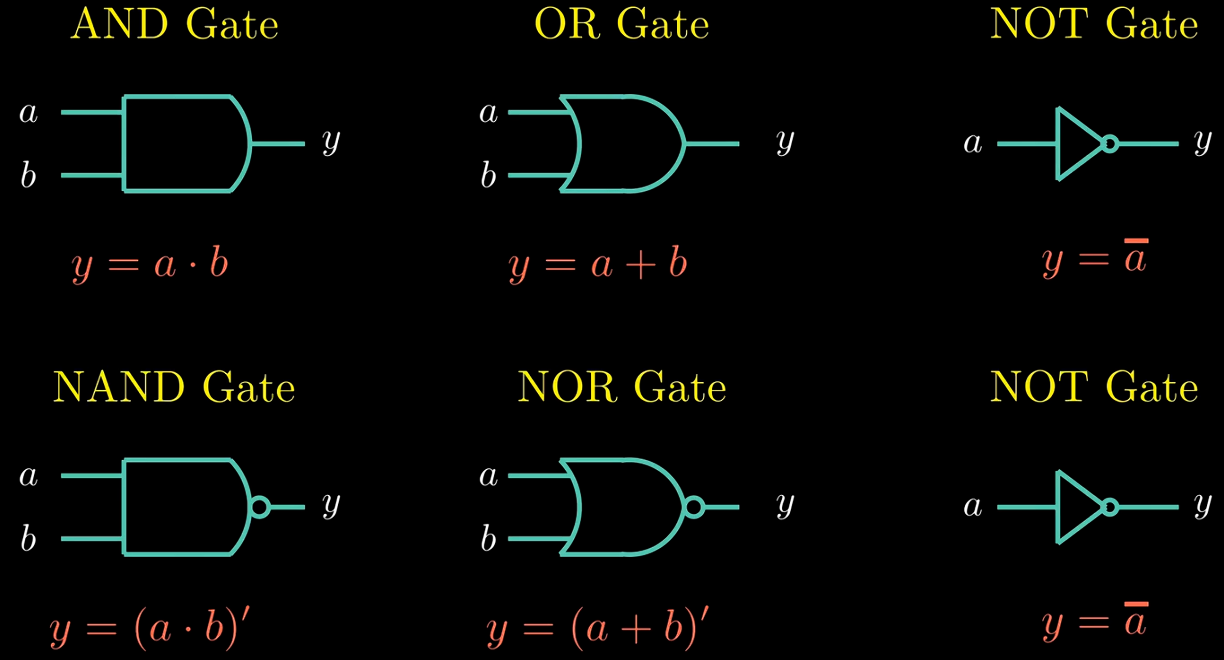
Logic Gate
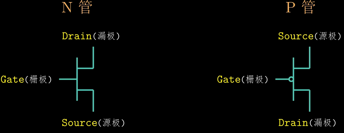
CMOS
Process
For Y86-84 :
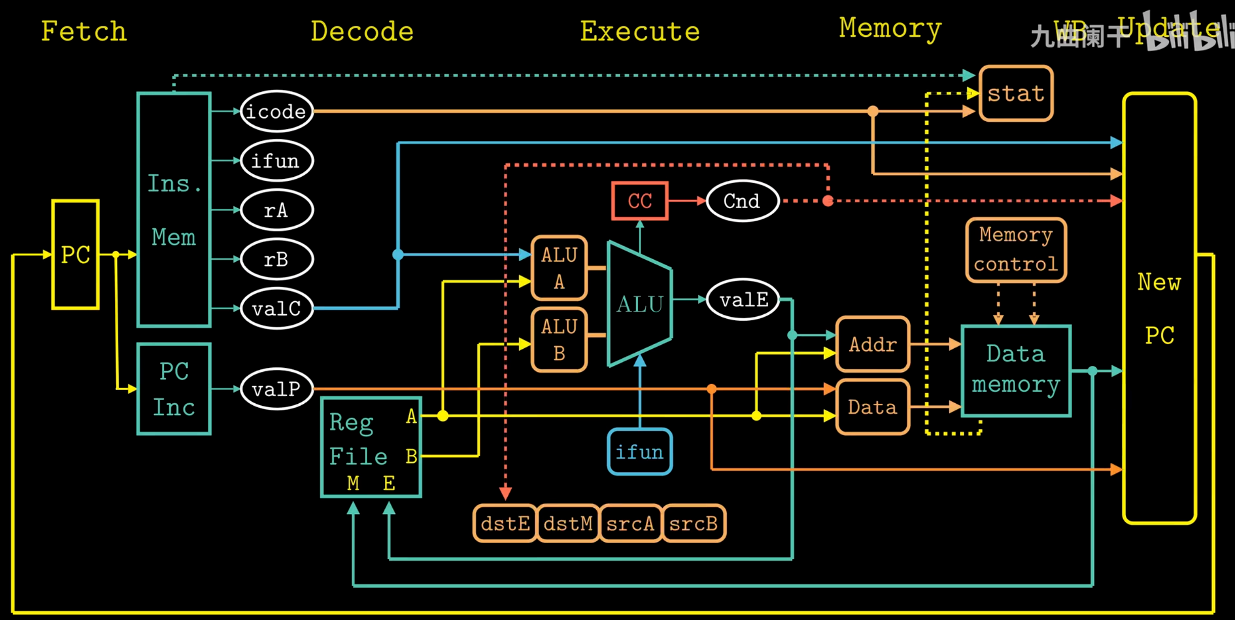
-
Fetch
- Read instruction bytes from memory using PC:
icode:ifun(instruction specifier)rA, rB(register specifiers)valC(8-byte constant)
- Compute next instruction address →
valP
- Read instruction bytes from memory using PC:
-
Decode
- Read up to two operands from registers
rA, rB→valA, valB- For
popq,pushq,call,ret: also read from%rsp
-
Execute
- Compute (ALU/address/stack) →
valE - Set condition codes
- Conditional moves: check CC, update dest register
- Jumps: decide branch
- Compute (ALU/address/stack) →
-
Memory
- Write to memory
- Read from memory →
valM
-
Write Back
- Write up to two results to registers
-
Update
- Set PC to next instruction address
Pipelining
-
Throughput the number of instructions in one second.
GIPS: Giga-Instructions Per Second
-
Circuit Retiming
Repositions registers within a design to optimize performance or area, without altering the system’s input/output behavior. It changes the state encoding by moving delays (registers) across combinational logic elements.
Hazards
The dependency between instructions may lead to incorrect computation results.
Data Hazards
-
Stalling
Stalling prevents data hazards by pausing the pipeline until required operands are ready. This approach is simple but reduces performance.
-
Data Forwarding (Bypassing)
Data forwarding allows a result computed in a later pipeline stage to be passed directly to an earlier stage as a source operand.
-
Load/Use Hazards
A load/use hazards occurs when an instruction requires a value that is still being loaded from memory by the previous instruction. Since the memory read completes late in the pipeline, forwarding cannot resolve the dependency in time, causing a stall.
Control Hazards
Control hazards occur when the processor cannot determine the next instruction's address during the fetch stage. In a pipelined processor, this typically happens for ret instructions and mispredicted conditional jumps.
-
retInserting bubbles to wait for the return address to be determined. -
Conditional Jump Branch mispredictions are handled by cancelling the erroneously fetched instructions through the insertion of pipeline bubbles (or via instruction squashing) in the decode and execute stages.
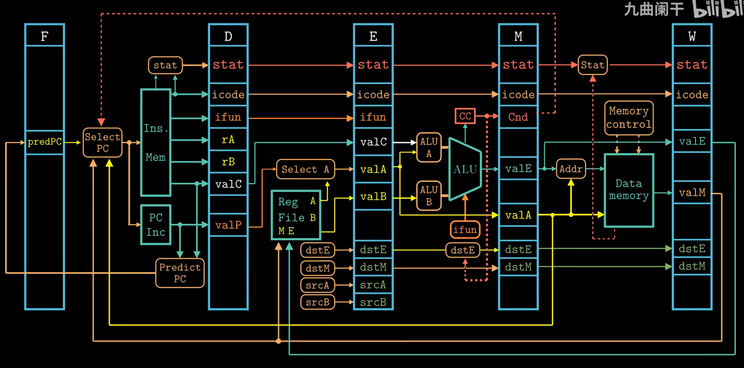
Pipelined Y86-64 Implementations
Fetch Stage
- Sequential Execution
halt, nop, rrmovq, irmovq , mrmovq, Opq, pushq, popq, covXX, addq
- Jump Execution
call, jxx (The Select PC mechanism is employed to correct branch mispredictions.)
ret
Decode Stage
The selection logic chooses between the merged valA/valP signals and one of five forwarding sources (e_valE, m_valM, M_valE, W_valM, or W_valE) based on the instruction type and hazard detection. If no forwarding is triggered, d_rvalA (the register file read) is used as the default value.
Pipeline Control Logic
-
Stall
Keep the state of the pipeline registers unchanged. When the stall signal is set to 1, the register will retain its previous state.
-
Insert Bubbles
Setting the state of the pipeline registers to a value equivalent to a
nopinstruction. When the bubble signal is set to 1, the state of the register will be set to a fixed reset configuration.
Load/Use Data
A one-cycle pipeline stall is required between an instruction that reads a memory value in the execute stage and a subsequent instruction that uses that value in the decode stage.
Mispredicted Branches
When a branch is mispredicted as taken, the pipeline must squash the incorrectly fetched instructions from the target path and redirect fetching to the correct fall-through address.
Processing ret
The pipeline must stall until the ret instruction reaches the write-back stage.
Exception Handling
When an instruction triggers an exception, all subsequent instructions must be prevented from updating programmer-visible state, and execution must halt once the exception-causing instruction reaches the write-back stage.
| Condition | F | D | E | M | W |
|---|---|---|---|---|---|
Handling ret | Stall | Bubble | Normal | Normal | Normal |
| Load/Use Hazard | Stall | Stall | Bubble | Normal | Normal |
| Mispredicted Branch | Normal | Bubble | Bubble | Normal | Normal |
Chapter 5 Optimizing Program Performance
Capabilities and Limitations of Optimizing Compilers
Memory Aliasing
The two pointers probably reference the same memory address.
Function Calls
Performance
CPE: Cycles Per Element.
Understanding Modern Processors
Instruction Control Unit (ICU) & Execution Unit (EU)
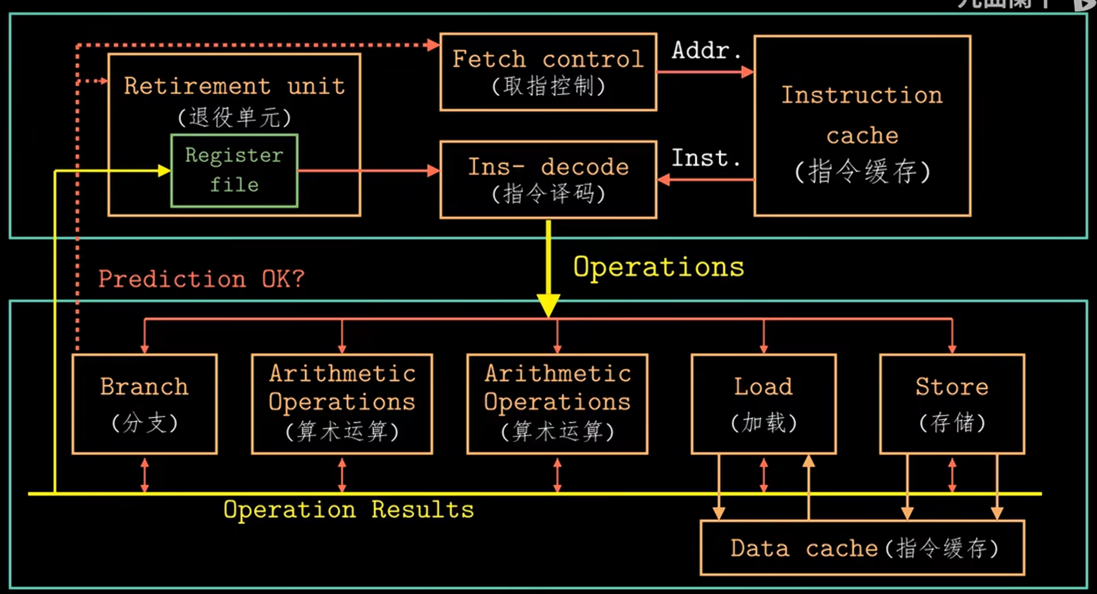
The ICU reads instructions from the instruction cache and uses branch prediction to speculatively fetch and decode future instructions in advance. This speculative execution mechanism allows the processor to start executing operations along the predicted program path before the actual branch outcome is known. If the prediction is incorrect, all speculative results are discarded and execution restarts from the correct branch target.
Decoded instructions are broken down into micro-operations, which are then sent to the EU for execution. The EU includes arithmetic units and dedicated load/store units, each with address calculation logic, to perform memory operations via the data cache.
All along, the retirement unit tracks instruction progress to ensure sequential program semantics are preserved. Instructions remain in a queue until their results are ready and all relevant branch predictions are verified. Only then are results committed to the architectural registers. If a branch was mispredicted, the affected instructions are flushed and their results discarded, preventing any erroneous state change in the program.
Register renaming allows out-of-order execution by assigning unique tags to instruction results. When a later instruction needs a register value, it uses the tag to get the result directly once ready, avoiding waits for register writes and enabling speculative execution.
Each operation is characterized by the following metrics:
-
latency It represents the total time required to complete the operation.
-
Issue time It indicates the minimum number of clock cycles needed between two consecutive operations of the same type.
-
Capacity It refers to the number of functional units capable of executing that operation.
CSC4303 Network Programming
Reference
Network Model
| Layer | Description | Example |
|---|---|---|
| Application | Programs that use network service | HTTP, DNS, CDNs |
| Transport | Provides end-to-end data delivery | TCP, UDP |
| Network | Send packets over multiple networks | IP, NAT, BGP |
| Link | Send frames over one or more links | Ethernet, 802.11 |
| Physical | Send bits using signals | wires, fiber, wireless |
Transport Layer
User Datagram Protocol (UDP)
-
Connectionless
Each packet is independent.
Sender Time Receiver | | |----- Packet1 -----> | | | |----- Packet2 -----> | | | -
Buffering
UDP buffering is a "temporary storage area" maintained by the operating system for each UDP port, where arriving packets queue up when applications can't process them immediately.
Application A Application B Application C ↓ ↓ ↓ [Port X] [Port Y] [Port Z] ← Port mapping ↓ ↓ ↓ [Queue 1] [Queue 2] [Queue 3] ← Independent UDP message queues │ │ │ └───────┬───────┴───────┬───────┘ ↓ ↓ [Port Multiplexer/Demultiplexer] ← Routes by port number ↓ [Incoming UDP packets] -
Header
Note that the Datagram length up to 64K.
     32-bit width (4 bytes per row)
0                  16                31
┌──────────────────┬──────────────────┐
│ Source Port      │ Destination Port │ ← Port addressing
│   (16 bits)      │   (16 bits)      │
├──────────────────┴──────────────────┤
│    Length        │    Checksum      │ ← Size & integrity
│    (16 bits)     │    (16 bits)     │
├─────────────────────────────────────┤
│                                     │
│           Application Data          │
│                                     │
└─────────────────────────────────────┘
Transmission Control Protocol (TCP)
-
Header
0 1 2 3 0 1 2 3 4 5 6 7 8 9 0 1 2 3 4 5 6 7 8 9 0 1 2 3 4 5 6 7 8 9 0 1 +-+-+-+-+-+-+-+-+-+-+-+-+-+-+-+-+-+-+-+-+-+-+-+-+-+-+-+-+-+-+-+-+ | Source Port | Destination Port | ← Identifies sockets +-+-+-+-+-+-+-+-+-+-+-+-+-+-+-+-+-+-+-+-+-+-+-+-+-+-+-+-+-+-+-+-+ | Sequence Number (32) | ← Byte-based sequencing +-+-+-+-+-+-+-+-+-+-+-+-+-+-+-+-+-+-+-+-+-+-+-+-+-+-+-+-+-+-+-+-+ | Acknowledgment Number (32) | ← Next expected byte +-+-+-+-+-+-+-+-+-+-+-+-+-+-+-+-+-+-+-+-+-+-+-+-+-+-+-+-+-+-+-+-+ | Data Offset | 0 | Flags | Window Size (16) | ← Control & flow control +-+-+-+-+-+-+-+-+-+-+-+-+-+-+-+-+-+-+-+-+-+-+-+-+-+-+-+-+-+-+-+-+ | Checksum (16) | Urgent Pointer (16) | ← Integrity & urgent data +-+-+-+-+-+-+-+-+-+-+-+-+-+-+-+-+-+-+-+-+-+-+-+-+-+-+-+-+-+-+-+-+ | Options (variable) | +-+-+-+-+-+-+-+-+-+-+-+-+-+-+-+-+-+-+-+-+-+-+-+-+-+-+-+-+-+-+-+-+ | Data | +-+-+-+-+-+-+-+-+-+-+-+-+-+-+-+-+-+-+-+-+-+-+-+-+-+-+-+-+-+-+-+-+-
Connection Establishment (Setup)
-
Three-Way Handshake
Both parties send Initial Sequence Numbers (ISNs) via SYNchronize segments. Each party acknowledges the other's sequence number using ACKnowledge segments.
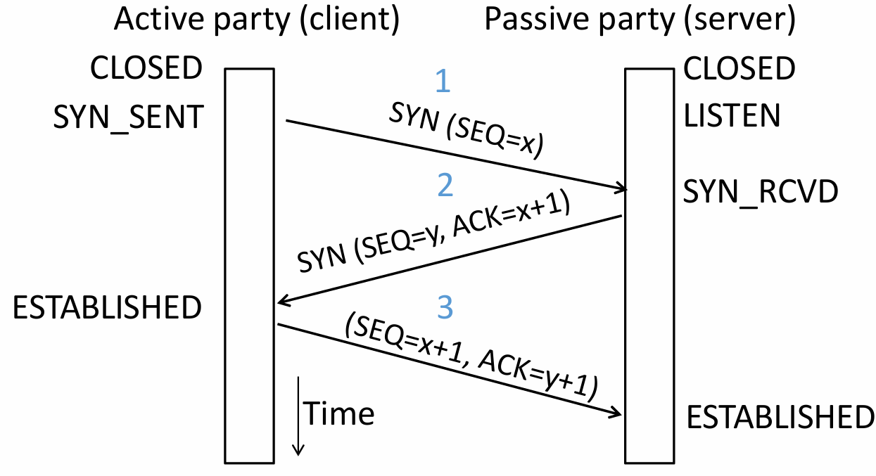
Step Initiator (Client) Receiver (Server) Description First Handshake Sends Waits for connection request Client requests to establish a connection and sends its ISN . Second Handshake Waits for acknowledgment Sends
It acknowledges receipt through sequence number .Server agrees to connect, sends its own ISN , and acknowledges the receipt of . Third Handshake Sends Connection established Client acknowledges the receipt of , and the connection is formally established. Three-way handshake prevents a server from wasting resources on stale or duplicate connection requests by requiring the client's final acknowledgment.
-
State Machine
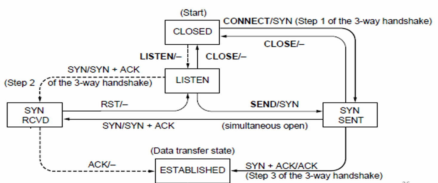
-
Client Path
CLOSED → connect() → SYN_SENT → Receive SYN+ACK → ESTABLISHED -
Server Path
CLOSED → listen() → LISTEN → Receive SYN → SYN_RCVD → Receive ACK → ESTABLISHED -
Both parties run instances of this state machine, and TCP allows for simultaneous open.
-
-
-
Connection Release (Teardown)
-
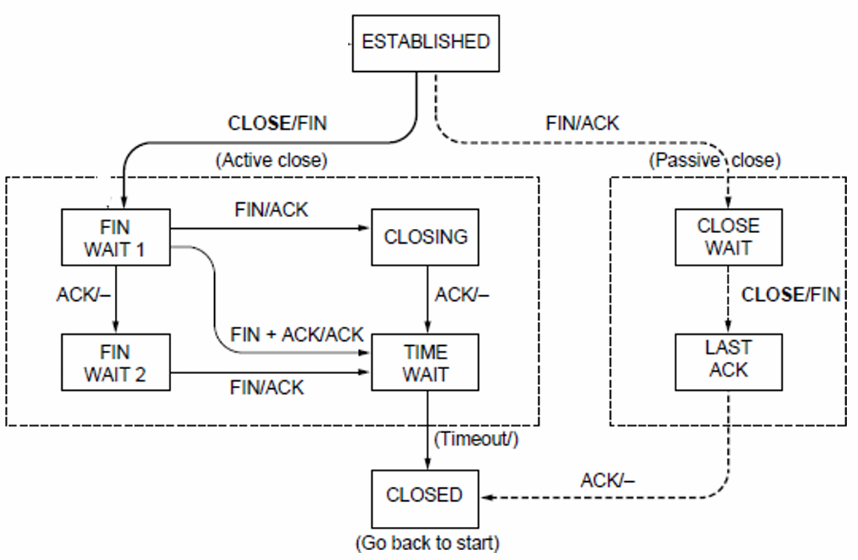
Four-Way Handshake (symmetric)
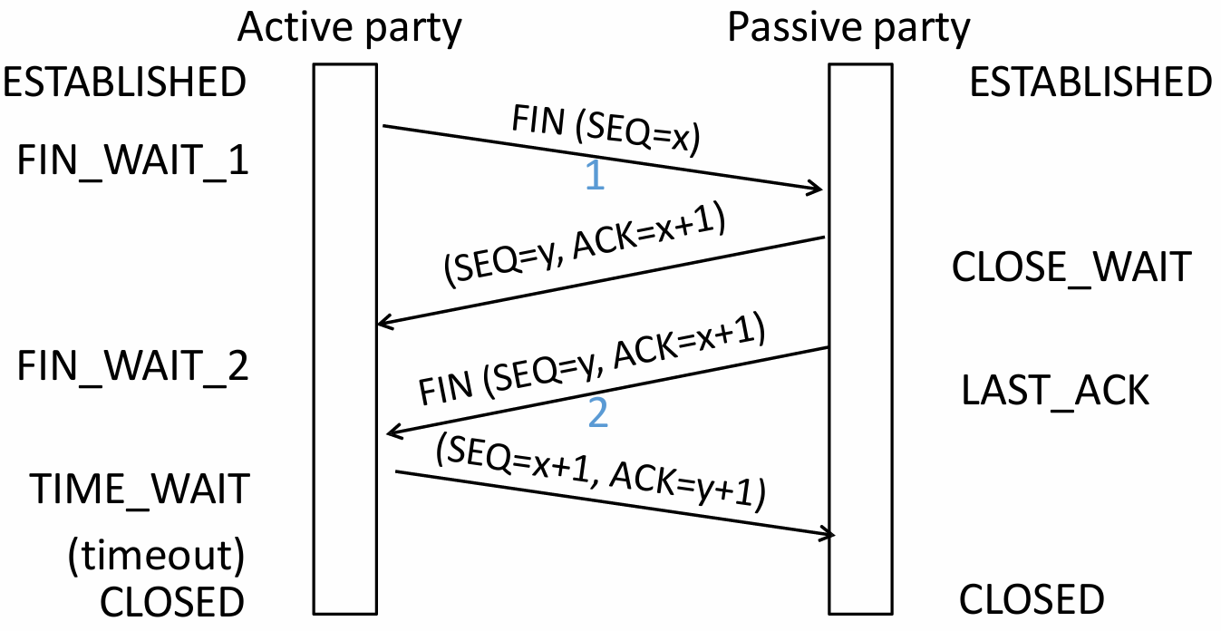
Step Initiator (Active Closer) Receiver (Passive Closer) Description First Wave Sends Waits for close request Initiator has finished sending data and requests to close its sending channel. Second Wave Waits for remaining data Sends Receiver acknowledges the close request but may still have data to send. Third Wave Waits for confirmation Sends Receiver has finished sending data and requests to close its sending channel. Fourth Wave Sends Connection closed Initiator acknowledges the close request. -
State Machine
-
Active Closer Path
ESTABLISHED → close() → FIN_WAIT_1 → Receive ACK → FIN_WAIT_2 → Receive FIN → TIME_WAIT → Timeout → CLOSED -
Passive Closer Path
ESTABLISHED → Receive FIN → CLOSE_WAIT → close() → LAST_ACK → Receive ACK → CLOSED -
TIME_WAIT State
-
(Maximum Segment Lifetime).
-
Lost ACKs can be recovered.
-
Old segments won't confuse new connections.
-
-
-
-
Flow Control (Receiver processing limitation)
-
Automatic Repeat Query
ARQ with one message at a time is Stop-and-Wait. It allows only a single message to be outstanding from sender.
-
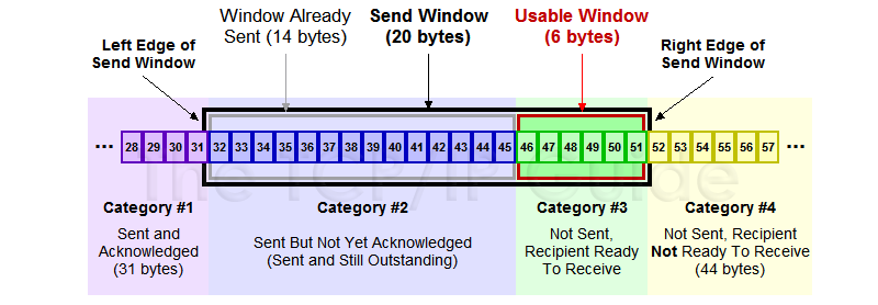
Sliding Window
It allows outstanding packets, enabling pipelining to send multiple packets per RTT for improved performance.
Sender buffers up to segments until they are acknowledged. The last frame sent minus last ack rec'd should no more than .
-
Go-Back-N
Only buffers next expected packet (LAS). Accepts only sequential packets, discards others, sends cumulative ACK.
-
Selective Repeat
Buffers entire window. Stores out-of-order packets, sends individual ACKs, retransmits only lost packets.
-
Sequence Number
bit counter wraps around at . Let be Last Acknowledgement Received, be Last Acknowledgement Sent.
Method Sender's Range Receiver's Range Min Number Needed to Avoid Overlap Go-Back-N Selective Repeat
-
-
Pacing
-
ACK Clocking (sender)
ACK clocking is a feedback mechanism where the network itself determines the sending pace, preventing queue buildup and ensuring efficient, low-latency data flow.
-
Flow Control (Receiver)
Flow control uses the
WINfield, calculated asWIN = ReceiveBuffer - (LastByteRcvd - LastByteRead), to dynamically limit the sender's window, preventing receiver buffer overflow.
-
Adaptive Timeout
Name Formula (average round‑trip time) (variability of RTT)
-
-
-
Congestion Control (Network capacity limitation) TCP congestion control uses a sliding window (cwnd), interprets packet loss as a congestion signal, and adjusts the window via AIMD to achieve an efficient and roughly fair bandwidth allocation.
-
Max-Min fairness
Increse the rate of one flow will decrease the rate of a smaller flow.
Step 1 Initialize all flows at zero
Step 2 Increase all flows equally
Step 3 Freeze bottlenecked flows
Step 4 Repeat for remaining flows -
Bandwidth allocation
Network layer provides direct feedback & Transport layer reduces load [Network is distributed, no single party has an overall picture of its state.]
-
Models
-
Open loop [reserve] & Closed loop [use feedback to adjust rates]
-
Host support & Network support
-
Window based & Rate based
TCP is a closed loop,host-driven, and window-based
-
-
AIMD(Additive Increase Multiplicative Decrease)
-
Hosts additively increase rate while network not congested
-
Hosts multiplicatively decrease rate when congested
-
-
-
TCP Tahoe/Reno
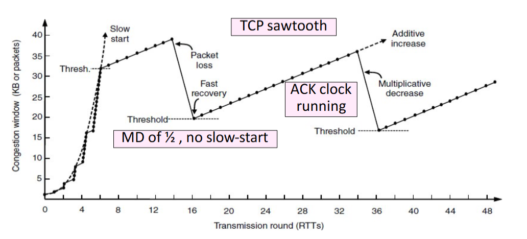
-
Slow Start
For each ACK received: , doubles every RTT.
-
Later Additive Increase (AI)
For each ACK received: , roughly adds 1 packet per RTT.
-
Switching Threshold (Initially Infinity)
Switch to AI when When , and after loss. Begin with slow start after timeout ().
-
Fast Retransmit
TCP's cumulative ACKs allow duplicate ACKs to signal lost packets for fast retransmission.(Treat three duplicate ACKs as a loss.)
-
Fast Recovery (TCP Reno)
Fast recovery keeps data flowing during retransmission by maintaining the ACK clock. It avoids resetting to Slow Start after packet loss. Set and then continue AI directly.
-
-
-
UDP & TCP
| Feature | TCP | UDP |
|---|---|---|
| Mode | Connections | Datagrams |
| Reliability | No loss, no duplicates, in-order delivery | May lose, reorder, or duplicate packets |
| Data Size | Unlimited | Limited |
| Flow Control | Flow control matches sender to receiver | Send regardless of receiver state |
| Congestion Control | Congestion control matches sender to network | Send regardless of network state |
| Example | Files, Web pages | Voice, video, DNS |
Socket
An endpoint for network communication that allows an application to attach to a specific port on the local network interface, enabling data exchange with other applications across the network.
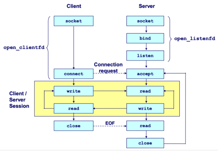
-
Process
Cilent
socket () ------------------------> connect () -> I/O -> close ()Server
socket () -> bind () -> listen () -> accept () -> I/O -> close ()-
The server blocks in
accept()onlistenfdfor incoming connections. -
The client calls
connect()to initiate the TCP handshake, which also blocks. -
Upon completion, the server's
accept()returns aconnfdand the client'sconnect()returns, establishing a bidirectional channel betweenclientfdandconnfd.
-
-
Create
int socket (int domain, int type, int protocol);-
domain AF_INET IPv4 / AF_INET6 IPv6.
-
type SOCK_STREAM TCP / SOCK_DGRAM UDP.
-
protocol 0 (automatically select the default protocol).
-
-
Bind
int bind (int sockfd, sockaddr *addr, socklen_t addrlen);When a server binds a socket to a specific address, it establishes that data arriving at that address is read from this socket, and data written to this socket is sent from that address.
-
socket address
struct sockaddr { uint_16 ss_family; // protocol family char ss_data[14]; // address data } -
sockaddr_in
struct sockaddr_in
{
    uint16_t sin_family; // always AF_INET
    uint16_t sin_port; // in network byte order
    struct in_addr sin_addr; // in network byte order
    unsigned char sin_zero[8]; // pad to sizeof (struct sockaddr), placeholder
}
Network data is transmitted in big-endian byte order. Use
htons()andhtonl()to convert host-ordered values into network-ordered short and long integers, respectively.
-
-
Listen
int listen (int sockfd, int backlog);listen ()transforms a socket descriptor into a listening socket capable of accepting client connections. Thebacklogparameter suggests how many pending connections the kernel may queue before refusing new requests (typically around 128). -
Accept
int accpet (int listenfd, sockaddr *addr, int *addrlen);accept()blocks until a client connects vialistenfd, stores the client's address inaddr, and returns aconnfdfor communication using standard Unix I/O functions. -
Connect
int connect (int clientfd, sockaddr *addr, socklen_t addrlen);Attempts to establish a connection with server at socket address
addr.To convert a string-formatted IP address (e.g.,
SERVER_IP), useinet_pton (int af, const char *src, void *dst)to transform it into binary network format.Feature listenfdconnfdPurpose Accepts connection requests Handles data exchange with a client Creation Once at server start Per accepted connection Lifetime Entire server runtime Duration of client service Quantity One per port One per active client Concurrent Use Listens for all clients Dedicated to single client -
Send and Receive
ssize_t read (int fd, void *buf, size_t len);returns the number of bytes actually read (0 indicates the connection is closed, -1 indicates an error).ssize_t write (int fa, const void *buf, size_t len);returns the number of bytes actually written (-1 indicates an error). -
Close
int close (int sockfd) -
Concurrency
-
Threading/Process Race conditions increase complexity!
-
I/O Multiplexing
-
select() -
poll()poll()is a system call used to monitor multiple file descriptors concurrently for I/O readiness. Unlikeselect(), it imposes no fixed limit on the number of file descriptors that can be monitored.struct pollfd { int fd; // file descriptor short events; // requested events short revents; // returned events }
-
-
Network Layer
Internet Protocol (IP)
- IPV4 Header
0                   1                   2                   3
0 1 2 3 4 5 6 7 8 9 0 1 2 3 4 5 6 7 8 9 0 1 2 3 4 5 6 7 8 9 0 1
+-+-+-+-+-+-+-+-+-+-+-+-+-+-+-+-+-+-+-+-+-+-+-+-+-+-+-+-+-+-+-+-+
|Version| IHL   |Type of Service|        Total Length (16)      | ← Basic identification (IHL : Header)
+-+-+-+-+-+-+-+-+-+-+-+-+-+-+-+-+-+-+-+-+-+-+-+-+-+-+-+-+-+-+-+-+
|        Identification (16)    |Flags|   Fragment Offset (13)  | ← Fragmentation control
+-+-+-+-+-+-+-+-+-+-+-+-+-+-+-+-+-+-+-+-+-+-+-+-+-+-+-+-+-+-+-+-+
|  Time to Live |    Protocol   |        Header Checksum (16)   | ← Routing & integrity (Time to Live : TTL)
+-+-+-+-+-+-+-+-+-+-+-+-+-+-+-+-+-+-+-+-+-+-+-+-+-+-+-+-+-+-+-+-+
|                       Source Address (32)                     | ← Sender IP
+-+-+-+-+-+-+-+-+-+-+-+-+-+-+-+-+-+-+-+-+-+-+-+-+-+-+-+-+-+-+-+-+
|                    Destination Address (32)                   | ← Receiver IP
+-+-+-+-+-+-+-+-+-+-+-+-+-+-+-+-+-+-+-+-+-+-+-+-+-+-+-+-+-+-+-+-+
|                    Options (if any, variable)                 | ← Optional features
+-+-+-+-+-+-+-+-+-+-+-+-+-+-+-+-+-+-+-+-+-+-+-+-+-+-+-+-+-+-+-+-+
|                           Payload (Data)                      |
+-+-+-+-+-+-+-+-+-+-+-+-+-+-+-+-+-+-+-+-+-+-+-+-+-+-+-+-+-+-+-+-+
-
IP Addresses An IP address is assigned to each network interface. Consequently, routers possess multiple interfaces, while most hosts have just one or two (wired and wireless).
-
IP Prefixes In a prefix of length L, the top L bits are identical across all addresses. In CIDR notation, such a prefix is denoted as
IP address/prefix length(e.g.128.13.0.0/16is128.13.0.0to128.13.255.255.) -
IP Forwarding It uses longest prefix matching to select the most specific route.
-
IP fragmentation
- MTU Max Transfer Size
- MSS Maximum Segment Size
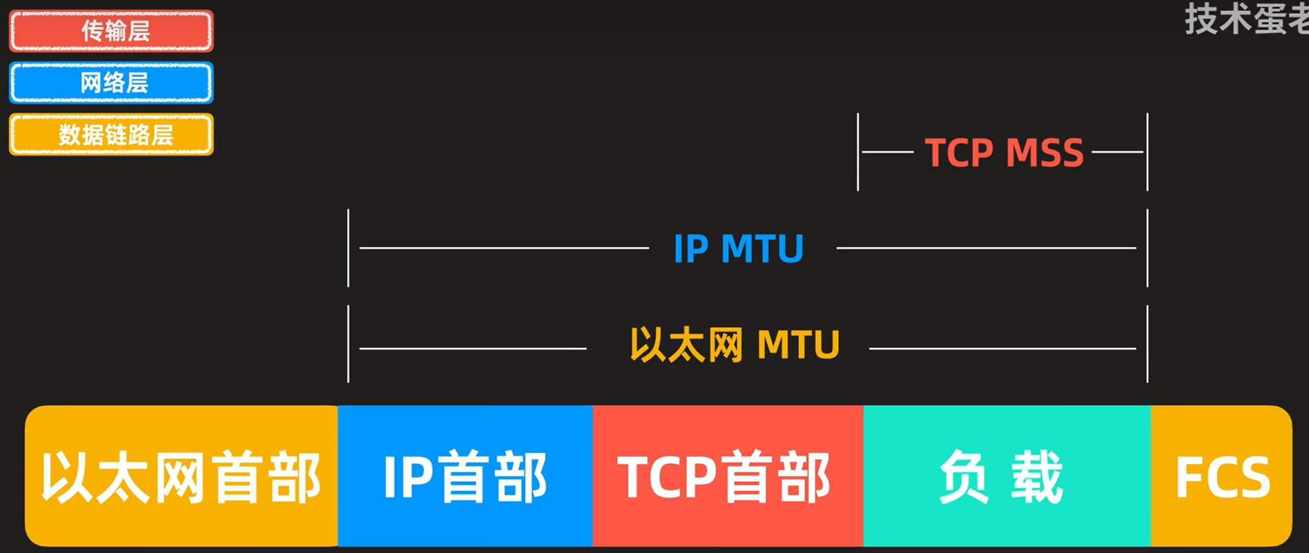
Each fragment is encapsulated with its own IP header.
Field Size (bits) Purpose Identification 16 Unique identifier for the original datagram; all fragments of the same datagram share this value. Flags 3 Control bits for fragmentation
DF (Don't Fragment) If set 1, routers must not fragment the packet.
MF (More Fragments) If set 1, more fragments follow, otherwise indicates that it is the last fragment.Fragment Offset 13 Indicates the position of this fragment's data in 8‑byte units relative to the start of the original datagram.
Dynamic Host Configuration Protocol (DHCP) [Application Layer]
Uses UDP ports 67 (server) and 68 (client).
| Step | Message | IP Header (Src → Dst) | Ethernet (Src → Dst) | Purpose |
|---|---|---|---|---|
| 1 | DISCOVER | 0.0.0.0 → 255.255.255.255 | Client MAC → FF:FF:FF:FF:FF:FF | Client broadcasts to find DHCP servers |
| 2 | OFFER | Server's IP → 255.255.255.255 | Server MAC → Client MAC | Server proposes IP configuration |
| 3 | REQUEST | 0.0.0.0 → 255.255.255.255 | Client MAC → FF:FF:FF:FF:FF:FF | Client accepts the offer |
| 4 | ACK | Server's IP → 255.255.255.255 | Server MAC → Client MAC | Server confirms and finalizes lease |
Address Resolution Protocol (ARP)
Every network device possesses a unique MAC (Media Access Control) address, which operates at the link layer.
ARP resolves IP to MAC addresses locally. A node broadcasts an ARP request, receives a private reply, and caches the mapping in its ARP table.
Internet Control Message Protocol (ICMP)
When an error occurs, an ICMP error report is sent back to the source IP address and the problematic packet is discarded. The source host must then rectify the issue.
-
Message Format
-
IP Header
Src = router, Dst = A, Protocol = 1 -
ICMP Header
Type = X, Code = Y -
ICMP Data
Src = A, Dst = B, ...
-
-
Type
| Name | Code | Usage |
|---|---|---|
| Dest. Unreachable (Net or Host) | 3/0 or 3/1 | Lack of connectivity |
| Dest. Unreachable (Fragment) | 3/4 | Path MTU Discovery |
| Time Exceeded (Transit) | 11/0 | Traceroute () |
| Echo Request or Reply | 8/0 or 0/0 | Ping |
- Traceroute
Traceroute sends probe packets with incrementing TTL. Each router that decrements TTL to zero replies with an ICMP Time Exceeded error, revealing its address.
Network Address Translation (NAT)
NAT maps multiple private IP:port pairs to a single public IP with unique external ports via a stateful translation table, enabling many internal devices to share one external address.
Routing and Forwarding
-
Fully Distributed Routing
- No central controller All routers are equal and make independent decisions.
- Local knowledge only Routers learn about the network by exchanging messages with directly connected neighbors.
- Concurrent operation
- Failure tolerance There may be node/link/message failures.
-
Hierarchical Routing
Introduce a larger routing unit. Route first to the region, then to the IP prefix within the region.
-
Routing Table
- Static Routing
- Dynamic Routing RIP (Routing Information Protocol), OSPF (Open Shortest Path First), BGP (Border Gateway Protocol).
-
IP Prefix Aggregation and Subnets (Longest prefix matching)
Routers can change prefix lengths without affecting hosts.
- Subnetting Split large prefix into smaller ones internally.
- Aggregation Join small prefixes into one large prefix externally.
-
Routing
-
Sink Tree
Sink tree for a destination is the union of all shortest paths towards the destination. Each node only stores next hop (parent) towards root.
-
Distance Vector Routing
Each node shares distance vectors with neighbors, updates paths using shortest heard distance, and forwards via best next hop.
Slow convergence, count-to-infinity, and routing loops occur because nodes only know neighbor info, not full topology, causing outdated routes to propagate and persist.
- RIP (Routing Information Protocol)
-
Link-State Routing
- Flooding
- Send an incoming message on to all other neigbors.
- Remember the message so that it is only flooded once.
- Dijkstra
- Flooding
Application Layer
Peer to Peer
Leverage peer resources: computation, storage, bandwidth. Also emerging: mobility, coins (tokens), sensors. Decentralized, scalable architecture.
Storage networks replicate files anywhere, making search difficult, especially with node churn.
-
Framework
- Join How to start participating
- Publish How to advertise files
- Search How to find files
- Fetch How to retrieve files
-
Napster
Server does all porcessing & Server maintains state & Single point of failure
- Join Client contacts central server on startup
- Publish Reports list of files to central server
- Search Query server → returns peer storing requested file
- Fetch Get file directly from peer
-
Gnutella
Complete decentralization & Query flooding
Search scope is & Unpredictable search time & No guarantee of finding files (TTL-limited search only works well for haystacks)
- Join Client contacts a few existing nodes on startup → these become its "neighbors"
- Publish No need (no central index)
- Search Ask neighbors → neighbors ask their neighbors → when/if found, reply back along the path; TTL limits propagation
- Fetch Get file directly from peer
-
Gnutella/KaZaA [Two-level hierarchy]
Kept a centralized registration
Supernodes have better connection to Internet and act as temporary indexing servers for other nodes to help improve the stability fo the network.
Standard nodes connect to supernodes and report list od files.
| Dimension | Napster | Gnutella | Gnutella/KaZaA (Two-Layer) |
|---|---|---|---|
| Index | Central server | No index | Supernodes maintain index (temporary central) |
| Search | Query central server | Flooding (ask neighbors) | Flooding between supernodes |
| Transfer | Direct peer-to-peer | Direct peer-to-peer | Direct peer-to-peer |
| Join | Contact central server | Find a few neighbors | Find and connect to a supernode |
-
BitTorrent
Central tracker server needed to bootstrap swarm.
- File swarming Files split into chunks; download from multiple peers, upload to others simultaneously.
- Tracker Central server coordinates peers (joins, maintains lists), but doesn't store files.
- Tit-for-tat Upload to the fastest peers you download from. Encourages fairness, discourages freeloading.
- Optimistic unchoke Randomly let new peers download to prevents starvation, discovers better partners.
- Rarest first Prioritize distributing scarce chunks to improve file availability and resilience.
- Out-of-band search Find files via Google/torrent sites. Scalable, no single point of failure.
-
DHT (Distributed Hash Table)
Decentralized system using consistent hashing: keys and nodes hashed onto a ring (Chord). Each key stored on its successor node. Finger tables enable lookup (Entry which starts from points to the first node on the ring that is ), improving from naive .
Amazon Dynamo
-
Architecture
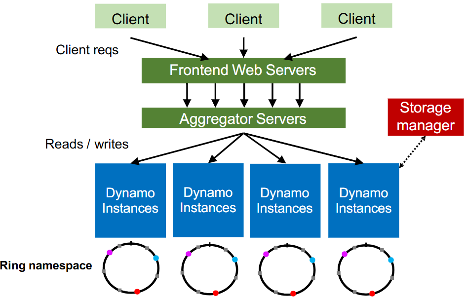
-
Partition
-
Hash partitioning
partition = hash(key) % partition_count -
Consistent hashing (better)
-
Virtual nodes (vnodes) Virtual nodes assign multiple ring positions to each physical node, distributing data migration and improving load balancing across all nodes.
-
Heterogeneity More powerful nodes can have more capacity, thus more vnodes.
-
Replication Dynamo skips nodes to ensure replicas reside on different nodes (set Replication Factor, i.e. ).
-
Dynamo Reads/Writes is configurable. When , the read and written will overlap, with last write wins (LWW) resolving conflicts.
-
Dynamo API
get (k)returns value(s) and context. It returns multiple versions if conflicts exist. The context contains Timestamps to track version history.put (k,context,value)uses the provided context to indicate which previous version(s) this new version supersedes or merges.
-
HyperText Transfer Protocol (HTTP)
- Request
| Method | Description |
|---|---|
| Read a Web page | |
| Read a Web page's header | |
| Append to a Web page | |
| Store a Web page | |
| Remove the Web page | |
| Echo the incoming request | |
| Connect through a proxy | |
| Query options for a page |
- Response
| Meaning | Example |
|---|---|
| Information | Server agrees to handle client's request Switching protocols |
| Success | Request succeeded New resource created No content present |
| Redirection | Page moved permanently Temporary redirect Cached page still valid |
| Client error | Bad request Authentication required Forbidden page Page not found Too many requests |
| Server error | Internal server error Bad gateway Service unavailable, try again later Gateway timeout |
-
Page Load Time (PLT)
PLT measures web performance from click to page visible, influenced by page structure, HTTP/TCP protocols, and network RTT/bandwidth.
HTTP/1.0 used one TCP connection per web resource.
-
Parallel Connections Browser runs multiple parallel HTTP instances, pulls in completion time of last fetch.
-
Persistent Connections Parallel connections compete with each other for network resources. Make one TCP connection to one server and use it multiple HTTP requests.
-
-
Web Caching and Proxies
-
Cached Content
- Locally expiry information (expires header) & heuristics (cacheable, fresh, not modified recently) [Content is then available right away]
- Server Last-Modified header & ETag” header [Content is available after 1 RTT (if connection open)]
-
Web Proxies Place intermediary between clients and server.
-
Domain Name System (DNS)
DNS is a naming service to map between host names and their IP addresses (Distributed directory based on a hierarchical namespace and automated protocol to tie pieces together).
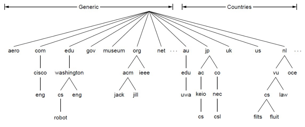
-
Top-Level Domains (TLDS)
-
DNS Resolution Start with the root nameserver and work down zones.
-
Local Nameservers and Root Nameservers
Local nameservers handle client queries and recursion, while root nameservers direct them to the appropriate top-level domain servers.
Root (dot) is served by 13 server names (
a.root-servers.nettom.root-servers.net) -
Caching Cached data periodically times out (set appropriate TTL).
-
DNS Security Extensions (DNSSEC)
To spoof, Trudy returns a fake DNS response that appears to be true.
- RRSIG for digital signatures of records
- DNSKEY for public keys for validation
- DS for public keys for delegation
Content Delivery Networks (CDNs)
A CDN uses DNS to direct each client to the nearest replica server based on their IP address.
Remote Prcedure Call (RPC)
-
Interface description languague Mechanism to pass procedur parameters and return values in a machine-independent way (use IDL compier, marshal and unmarshal).
-
At-Least-Once Scheme Upon timeout, the client stub retransmits the request. After several failed attempts, it returns an error.
-
At-Most-Once Scheme
Since identical calls may come from different clients, duplicate detection requires a unique xid per request.
The client includes "seen all replies " with every RPC, allowing the server to discard outdated xids and prevent unbounded state growth.
A pending flag per executing RPC avoids re-running duplicates.
To survive crashes, both client and server persist pending/completed RPCs to disk.
-
Exactly-Once retransmission (At-Least-Once) + deduplication (At-Most-Once) + persistence on both sides for crash recovery. Limitation: not possible with external physical actions.
Distributed Storage System
-
The Google File System (GFS)
-
Target environment
- Files are huge, but not many.
- Write once, read many.
- I/O bandwidth is more important than latency.
Typical workloads : Bulk Synchronous Processing (BSP).
-
Design Decisions
-
Chunk Use 64MB chunks amortize seek costs, approach disk transfer limits for streaming workloads, and reduce both metadata overhead on the master and RPC overhead for large reads/writes.
-
Replication Replicate each chunk three times across racks, with one replica in the same rack for low write latency and two or more in other racks for fault tolerance against rack-level failures, trading off cross-rack bandwidth.
-
Single master Centralize metadata only to avoid making the master a bottleneck, while keeping data transfer peer-to-peer between clients and chunkservers to maximize throughput and scalability.
-
Record append Support concurrent appends.
-
-
General Architecture
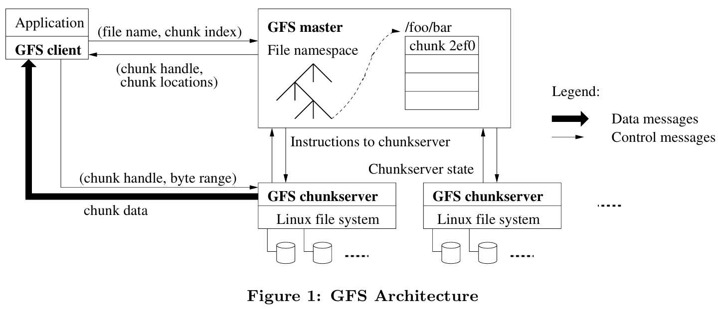
-
Single master
Shadow masters provide read-only access with slightly stale metadata by replicating the primary's operation log, ensuring availability during primary failure.
GFS prevents master overload by minimizing its involvement: data never passes through it, large chunks reduce metadata ops, and chunk leases delegate write coordination authority to primary replicas.
Category Responsibility Description Regular Management Metadata Storage Stores namespaces, file-to-chunk mappings, chunk locations in memory. Namespace Locking Locks directory operations to handle concurrent accesses. Periodic Communication Heartbeats with chunkservers to monitor health and exchange state. Chunk Lifecycle Creates chunks (rack-aware); re-replicates when replicas low; rebalances load/space. Background Cleanup Garbage Collection Logs deletion, renames files as hidden, lazily reclaims space. Stale Replica Deletion Uses version numbers to detect and remove outdated replicas. -
Metadata
- file and chunk namespaces
- mappings from files to chunks (unique ID)
- locations of each chunk’s replicas (ask for chunkserver)
-
Chunkserver Chunkservers store 64MB chunks locally with version numbers and checksums while clients read/write via chunk handle and byte range from master without data caching.
-
Client GFS client sends control requests to master, caches metadata, but transfers data directly to/from chunkservers without caching file data.
-
-
File read and write
- Read Client asks master for chunk locations, then reads data directly from the nearest chunkserver and returns it to the application (choose one to read).
- Write Client gets locations, pushes data to all replicas' buffers, then primary serializes writes and coordinates secondaries before acknowledging (write all primary and secondaries).
-
Fault Tolerance
GFS uses heartbeats to detect failures, reduces replica counts, and re-replicates chunks elsewhere to restore full replication.
-
Time in Distributed Systems
-
Cristian Algorithm
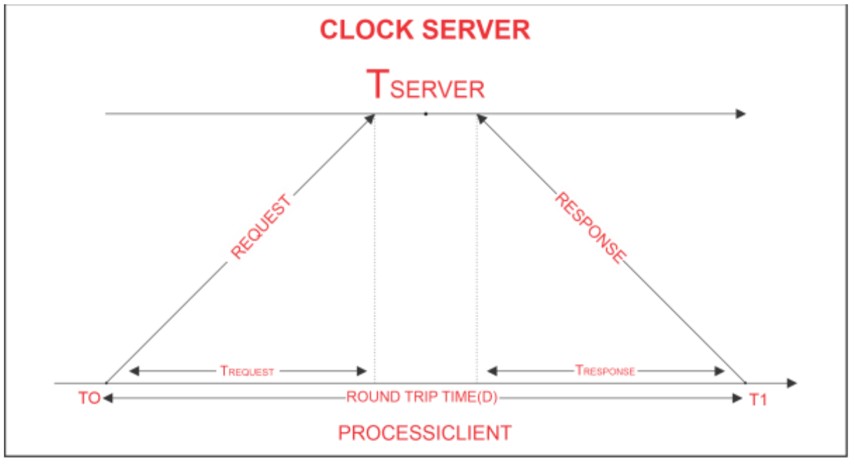
-
The Lamport Clock Algorithm
Lamport clocks ignore physical time and only capture the happens-before relationship between events.
Each process maintains a local clock . For a local event, , then . When process sending an message , set . When process receives an message , .
If , then . However, the converse does not hold — Lamport timestamps alone cannot be used to infer causal relationships between events.
-
Totally-Ordered Multicast
Totally-ordered multicast ensures identical processing order. Replicas sort queues by timestamps (dynamically updating the head), broadcast ACKs strictly for this head, and execute it once globally acknowledged.
-
Vector clock
Initially all vectors are .
For each local event on process , increment local entry .
If process receives message with vector , then , and increment local entry .
| Comparison | Lamport Clock | Vector Clock |
|---|---|---|
| Given | ||
| Conclusion | Either or | |
| Precision | Cannot distinguish causality from concurrency | Precisely captures happens-before relation |
Parallelism Basics and Collective Communication
-
Communication patterns
- Point-to-point communication
- Collective communication
-
Model
- Cost of Communication (or if a message encounters a link that simulaneously accommodates messages) ( Latency, Transfer time per byte, Message size in bytes)
- Primitive
Primitive Pattern Description Broadcast One-to-all One process sends the same data to all processes Reduce(-to-one) All-to-one All processes perform a reduction operation (sum, max, etc.) and send the result to one process Scatter One-to-all One process distributes distinct data chunks to all processes Gather All-to-one All processes send their data to a single process Allgather All-to-all All processes collect data from all processes (each process gets the full data set) Reduce-scatter All-to-all Perform local reduction first, then scatter results (first half of Allreduce) Allreduce All-to-all All processes perform a reduction operation, and the result is distributed to all processes
-
Minimum Spanning Tree Algorithm (emphasize low latency for small message)
Recursive halving broadcast splits nodes in half sends to opposite half recurses achieving rounds optimizing latency for small messages.
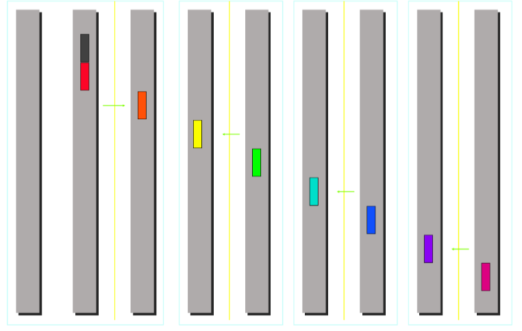
Totoal cost:
- Broadcast
- Reduce Compute overhead is required for reduce.
- Scatter/Gather
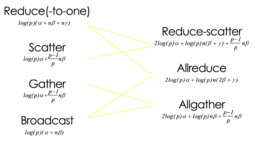
-
Ring Algorithm (emphasize bandwidth utilization for large message)
The bandwidth term now dominates.
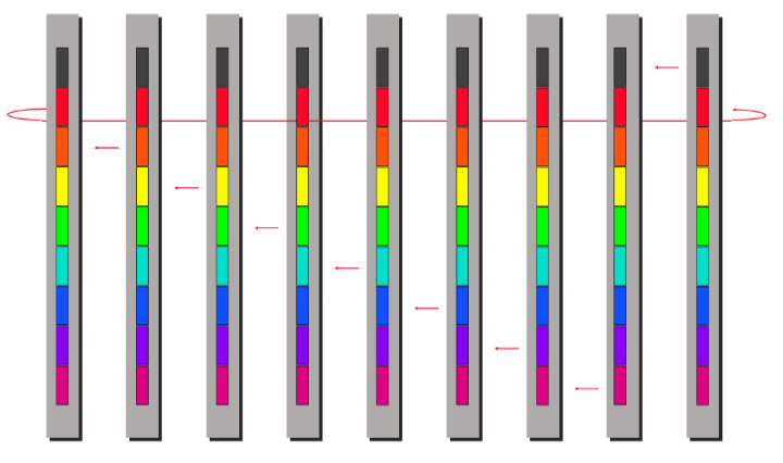
ring algorithm can not be better for Scatter and Gather.
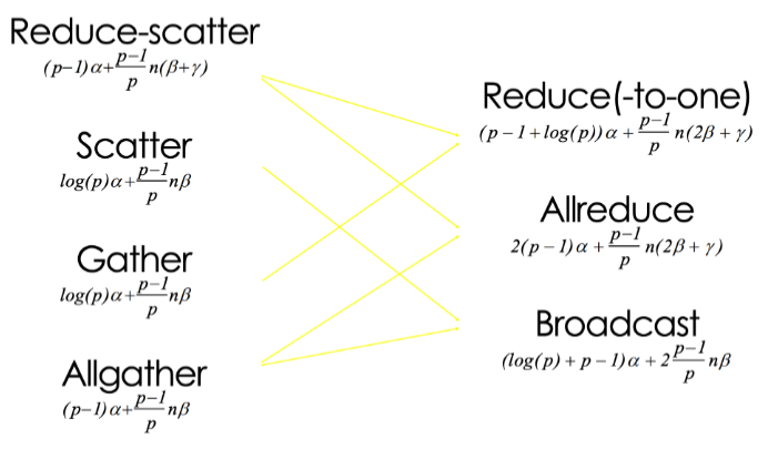
LLM
Parallelism in Distributed Machine Learning
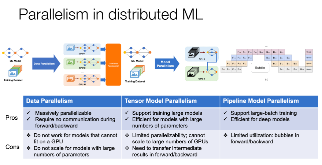
Continuous batching
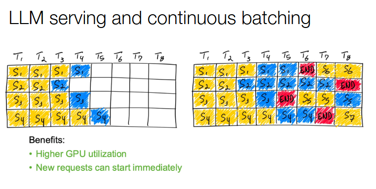
DDA3020 Machine Learning
Information Theory
Informaion
When , , which means there is no uncertainty, then no information.
Entropy
Entropy is defined as the expected value of information from a source.
Cross-entropy
Cross-entropy measures average bits needed to encode events from true distribution using estimated distribution .
Property 1
Proof
.
Property 2
Proof
By Jensen equality, for any convex function , .
Since is concave, we can implies Let , then The equality holds only when .
Kullback-Leibler divergence (KL-divergence)
The distance between two distributions.
Property 1
Proof
Property 2
Linear Regression
Modeling of Linear Regression
Deterministic Perspective
Find which minimizes the following expression:
Probabilistic Perspective
where is called obervation noise or residual error. The output can also be seen as a random variable, whose conditional probability is :
Given the training dataset , by maximum log-likehood estimaiton, we get
Solutions of Linear Regression
Analytical solution
Let , then
Differentiating with respect to and setting the result to :
If is invertible then
For linear regression with multiple outputs, , then
Gradient Descent
, can be updated by gradient descent algorithm:
Classification
Binary Classification
If is invertible then , .
Multi-Category Classification
Each ro in has a one-hot assignment, then If is invertible then , .
Linear Regression Models
Ridge Regression
where (The bias should not be normalized).
To get ,
Where is the identity matrix with the top-left element set to 0 to avoid penalizing the bias term .
We can assume that the parameter follow a zero-mean Gaussian prior (omit the bias ).
Utilizing this prior, we obtain the maximum a posteriori (MAP) estimation
Polynomial Regression
Note that is still a linear function .
Lasso Regression
, then we have .
Ridge uses L2 penalty, shrinking weights towards zero without feature selection. In contrast, Lasso uses L1 penalty, forcing some weights to exactly zero, achieving model sparsity and automatic feature selection.
Robust Linear Regression
Adpot the loss as follows .
Assuming that , .
Two ways to make it differentiable:
-
.
-
By using the following equation .
Then it can be reformulated as follows:
Given , ; Given , .
Comparison
| Regression Method | ||
|---|---|---|
| Gaussian | Uniform | Least squares |
| Gaussian | Gaussian | Ridge regression |
| Gaussian | Laplace | Lasso regression |
| Laplace | Uniform | Robust regression |
| Student | Uniform | Robust regression |
Logistic Regression
Hypothesis Function
The decision boundary satisfies when , and when , , it is determined by .
Cost Function
-
Loss
-
Linear Regression
,
-
Logistic Regression
-
-
Cross-entropy Loss
For , ,.
For , ,.
Gradient Descent
Assume samples in total. Learning by minimizing
By gradient descent
Multi-class Classification
Softmax
Cost Function
Regularized Logistic Regression
Linear Regression vs Logistic Regression
| Dimension | Linear Regression | Logistic Regression |
|---|---|---|
| Task Type | Regression task predicting continuous real values | Classification task predicting discrete class labels |
| Model Hypothesis | Linear function Output range | Sigmoid-mapped linear function Output range (posterior probability of positive class) |
| Loss Function | Residual sum of squares (MSE) | Cross-entropy loss |
| Solution Method | Closed-form solution or gradient descent | No closed-form solution, optimized via gradient descent |
Supoort Vector Machine
Larger Marigin
Denote is a hyperplane, then is orthogonal to the hyperplane, and has the distance to the hyperplane.
Margin is defined as the distance between the hyperplane and the closest data point, which can be formulated as with .
Since . Set , then ,
Then the optimization problem can be formulated as follows:
Hinge Loss
Let where be the hypothesis function, then the cost function can be defined as follows:
The hinge loss is defined as follows
Then the optimization problem can be reformulated as follows
Largrange Duality
The objective function of SVM is
Its Lagrangian function is defined as follows
The KKT conditions are as follows
Then the Largangian function can be reformulated as follows
Then the dual problem is obtained as follows
The data points with are called support vectors, which locate on the margin and determine the decision boundary. Let be the set of support vectors, then the decision boundary can be determined by any support vector as follows:
SVM with Slack Variables
In this case, the optimization problem can be formulated as follows
Its Lagrangian function is defined as follows
The KKT conditions are as follows
The the Lagrange function can be reformulated as follows
The dual problem can be reformulated as follows
Let . The bias parameter can be determined by any support vector with as follows
| Condition on | Slack | Contributes to classifier? | Correctly classified? | Location relative to margin / decision boundary |
|---|---|---|---|---|
| No | Yes | Outside the margin | ||
| Yes | Yes | On the margin | ||
| Yes | Yes | Inside the margin, not crossing decision boundary | ||
| Yes | No | Crossing decision boundary |
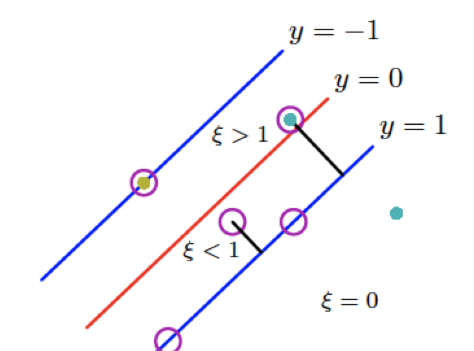
SVM with Kernels
Define the kernel function , then the dual problem can be reformulated as follows
The solution becomes
The prediction of new data becomes
Some kernel functions
Multi-class SVM
Predict the label of as , , use one-vs-rest strategy to train binary SVM classifiers.
Tree-based Methods
Decsion Tree
A decision tree (non-parametric model) is a hierarchical model for supervised learning whereby the local region is identified in a sequence of recursive splits.
Classification Tree
-
Impurity Measure (Choose the attribute that maximizes the reduction in impurity.)
Let be the seef of instances of belonging to class (), then is the proportion of class in .
Entropy is the measurement of impurity, which is defined as follows
And the entropy of given the condition of attribute is defined as follows (Suppose attribute to split into subsets )
Information gained by branching on atribute is defined as follows
-
Gini Index
Gini index is another measurement of impurity, which is defined as follows
It means the probability of different class labels for two randomly selected instances from .
And the Gini index of given the condition of attribute is defined as follows (Suppose attribute to split into subsets )
Gini gain by branching on atribute is defined as follows
Regression Tree
The regression tree grows by recursively selecting the binary split on any variable that most reduces the sum of squared errors.
is the prediction for leaf , where is the number of instances in leaf .
-
Mean Squared Error (MSE)
The total MSE is .
-
Sum of squared Errors (SSE)
The total SSE is .
Overfitting and Pruning
Pruning of the decision tree is one by replacing a subtree with a leaf node. The subtree is replaced if the error of the subtree on the validation set is larger than the error of the leaf node on the validation set.
Ensemble Models
Bagging
Sample records with replacement from the training set to create multiple bootstrap samples, and train a base model on each bootstrap sample. The final prediction is obtained by averaging the predictions of all base models.
It aggreates the predictions of all single trees and produces many correlated trees, which the diversity of the trees is not high.
Random Forest
It chooses a random subset of features to split each node, which increases the diversity of the trees and reduces the correlation between trees.
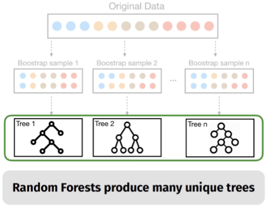
Neural Networks
Activation Function
Perceptron Model
, the objective function is , and the update rule is .
For a new data point , the prediction is , which is a linear classifier.
Multi-layer Feedforward Neural Networks
To solve XOR, a one‑hidden‑layer network learns non‑linear input features. Each layer re‑expresses the previous layer’s output, progressively extracting more abstract and discriminative features.
, where is the transformation of layer .
Backpropagation (using computational graph (CG))
Forward Pass
For each , compute as a function of its parents.
Backward Pass
, then for , . Also update parameters by
where is the cost function of layer .
Convolutional Neural Networks
Convolutional Layer
Input volume is .
A convolutional layer has four hyperparameters: number of filters , filter size , stride , and zero padding (per side).
Output spatial size is and .
Output volume is .
Number of parameters is weights plus biases. parameters is weights plus biases.
Pooling Layer
Pooling layer has no learnable parameters. Hyperparameters are filter size and stride .
Output spatial size is and .
Pooling operates on each channel independently, so output volume is .
Common pooling functions are and .
Fully Connected Layer
A fully connected layer computes the class scores, resulting in an output volume of , where is the number of classes, which contains neurons that connect to the entire input volume.
Recurrent Neural Networks and Transformer
RNN
Basic
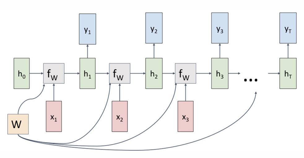
, , where is the transition function and is the output function. The cost/error function is , where .
However, the basic RNN suffers from vanishing/exploding gradient problem, which makes it difficult to learn long-term dependencies.
Long Short-Term Memory (LSTM)
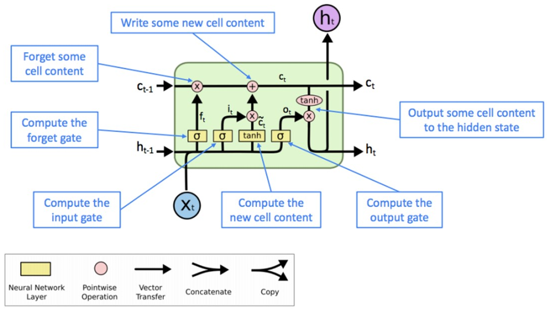
Limitations
- Difficulty with Long-Term Dependencies
- Limited Parallelization
Transformer
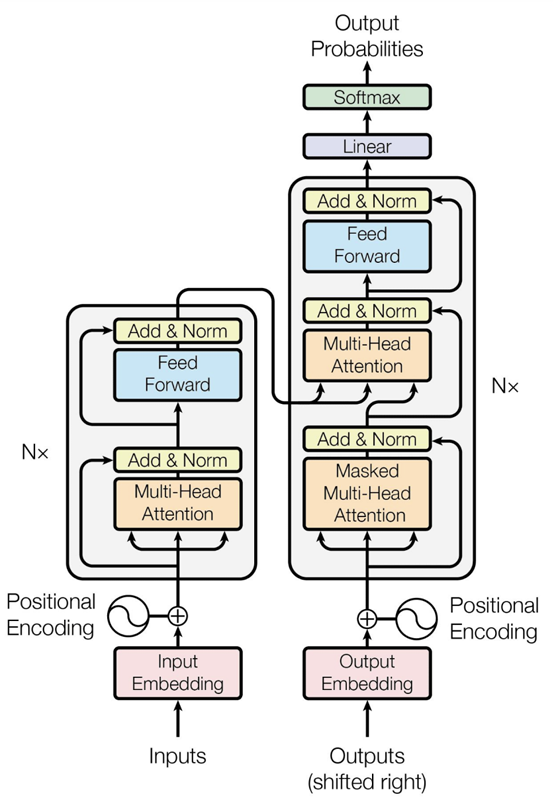
Attention Mechanism
Let be the query, key, and value matrices, where and is the input sequence. Then the attention output is defined as follows
Multi-head Attention
Multi-head attention allows the model to jointly attend to information from different representation subspaces at different positions, capturing diverse types of relationships in parallel.
Bias-variance Tradeoff
Let be training dataset drawn from , be the model trained by algorithm on .
-
expected test error for a fixed model .
-
expected test error for the algorithm .
-
the expected test error . (mean squared error (MSE))
Now decompose the second term , .
-
Comparsion
Term Description Variance Measures how much the predictions of a model vary when trained on different training sets. (model's sensitivity to the specific training data) Bias² Measures how far the average prediction of a model is from the true value. (model's systematic error) Noise Measures how much the observed values vary around the true target function due to randomness in the data. (data's inherent unpredictability) 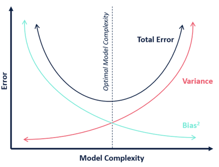
Performance Evaluation
Hyper-parameter Tuning
Determined typically outside the learning algorithms rather than earned by a learning algorithm based on the trainingset.
Cross-validation
Cross-validation is a statistical method of evaluating generalization performance that is more stable and thorough than using a split into a training and a test set.
-
K-fold cross validation
Split the train data into folds, try each fold as validation, while other folds as train. Note that is a hyper-parameter.
Evaluation Metrics
Regression
- Mean Square Error
- Mean Absolute Error
Classification
-
Confusion Matrix
Actual \ Predicted (Predicted) (Predicted) (Actual) (Actual) -
Accuracy The total number of correctly classified samples over all samples under evaluation.
-
Precision The proportion of correctly predicted positive samples among all samples predicted as positive.
-
Recall The proportion of correctly predicted positive samples among all actual positive samples.
-
Cost-sensitive Accuracy (different classes may have different importance)
-
Binary Classification
Metric Formula (True Positive Rate) (False Negative Rate) (True Negative Rate) (False Positive Rate) If positive and negative classes are balanced, then .
As the decision threshold varies from to , FPR decreases while FNR increases, and their intersection point where equals is called the Equal Error Rate (). The lower the , the better the classifier.
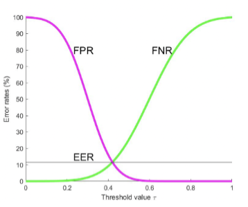
-
-
Receiver Operating Characteristic Curve (ROC) The relationship between FNR and FPR.
-
Area Under the ROC (AUC) The probability that a randomly chosen positive example is ranked higher than a randomly chosen negative example. (It means the perfect prediction if it equals to .)
Consider a set of binary samples indexed by for positive class, and for negative class. Let be a predictor and .
Consider also a Heaviside step function given by
Then AUC can be expressed by .
Unsupervised Learning
Clustering
Clustering is a problem of learning to assign labels to examples by leveraging an unlabeled dataset.
Dimensionality Reduction
Principal componentanalysis (PCA) is a technique that converts a set of observations of possibly correlated variables into a set of values of linearly uncorrelated variables, called principal components.
Density Estimation
Estimate the distribution based on some observed data.
-
Kernel Density Estimation (KDE)
where is a hyper-parameter called kernel size, which can be tuned using -fold cross-validation.
Autoencoder
An autoencoder is a type of artificial neural network used to learn efficient coding of unlabeled data.
Self-supervised Learning
Self-supervised learning (SSL) is a paradigm where a model learns from unlabeled data by automatically generating pseudo-labels from the data itself, without requiring human annotation.
K-means Clustering
Initialize centroids, assign each point to nearest centroid, update centroids by mean of assigned points, repeat until convergence.
In short, K-means will minimize the within-cluster variance, as follows:
where denotes is assigned to cluster .
Coordinate Descent
Assignment (Given to update )
Note that the assignment for each data can be solved independently, , pr
The solution can be obtained as follows
Refitting (Given to update )
Note that can be optimized independently, as follows
By setting the derivative as 0, ,
Since the objective function is non-convex, K-means may converge to a local minimum, and the final solution can be sensitive to the initial centroids. To mitigate this issue, it is common practice to run K-means multiple times with different random initializations and select the solution with the lowest within-cluster variance.
Performance Evaluation
Internal Evaluation Metrics (Silhouette Coefficient)
Define as the mean distance between a point and all other points in the same cluster. Define the smallest mean distance of a point to all points in any other cluster.
The silhouette coefficient for a single sample is formulated as follows:
close to indicates that the sample is well clustered.
External evaluation metrics (Rand Index)
| Symbol | Definition |
|---|---|
| same in , same in | |
| different in , different in | |
| same in , different in | |
| different in , same in |
For random clusterings, the expected value of the Rand Index is not zero. Let , and Adjusted Rand Index (ARI) is defined as follows:
Gaussian Mixture Models
where are the mixing coefficients, , , , and
Alternating Upadating Algorithm
Derivation from MLE
The log-likelihood is given by
Let the derivate of with respect to be zero:
Let , then
Let the derivate of with respect to be zero:
Considering the by using the Lagrange multiplier to handle the constraint . Maximize , then
Add a hidden variable to indicate which component generates , then the complete-data log-likelihood is given by
Algorithm
-
Initialize .
-
E-step Compute the responsibilities
-
M-step
First, compute the effective number of points assigned to component :
Then update the parameters:
-
Repeat steps 2 and 3 until convergence.
The Expectation-Maximization Algorithm
Jensen's Inequality
For a convex function , we have .
For a concave function , we have .
Proof (for convex function )
When , , , where . Then .
When , proof by induction applies. Assuming the inequality holds for variables, consider variables. The following relation holds Where . Then
Auxiliary Distribution of Latent Variables
Let denote the observed data, denote the latent variables. The log-likelihood can be expressed as follows:
Let be an auxiliary distribution over the latent variables and they are independent, , with constraint . Then by using Jensen's inequality, we have
To extend the above equation to the whole dataset, we have
E Step
Given , the optimal is given by
The optimal is given by , the KL divergence is going to be zero.
M Step
Given , the optimal is given by
Substituting got in E step into the above equation,
EM Convergence
Application to GMM
E-step computes the posterior responsibility of each Gaussian for each data point, and M-step updates the parameters using weighted averages based on those responsibilities.
Set , then compute the expected log-likelihood as follows:
Next, maximize this expected log-likelihood with respect to to obtain closed-form updates for the M-step.
Principal Component Analysis
Given a dataset , PCA aims to find a projection matrix that maps the original data to a lower-dimensional space while maximizing the variance of the projected data.
Projection onto a Subspace
Let and -dimensional subspace is spanned by an orthonormal basis . The projection of a data point onto the subspace is given by
The vector is orthogonal to the subspace , , .
Principal Component Analysis Algorithm
Variance Maximization
Since , the above equation can be rewritten as follows
Note that the following derivations are equivalent by the Pythagorean theorem
Define the empirical covariance matrix as follows
Then the optimization problem can be rewritten as follows
By using the Lagrange multiplier to handle the constraint :
where .
Then the optimal can be obtained by setting the derivative of with respect to as zero:
Utilizing the SVD decomposition of
where are the eigenvalues of , and is the corresponding eigenvector.
Substituting the SVD decomposition of into the above equation:
where is the set of indices corresponding to the eigenvectors and with .
The Uncorrelatedness of Coveriance Matrix of Projected Data
Let , .
The covariance matrix of the projected data is given by
Let , then , and is the top-left block of . Then
Then the covariance matrix of the projected data can be rewritten as follows
where is a diagonal matrix. Therefore, the covariance matrix of the projected data is diagonal, which means that the projected data are uncorrelated, , for .